Modelling eye-tracking data in comparative judgement

class: center, middle, inverse, title-slide

# Modelling eye-tracking data in comparative judgement
## ⚔<br/>EARLI SIG27 - 2020
### Sven De Maeyer; Marije Lesterhuis; Marijn Gijsen
### University of Antwerp
### 2020-11-25

---

name: introduction
class: center,inverse, bottom
background-image: url(sharon-mccutcheon-NeRKgBUUDjM-unsplash.jpg)
background-size: contain

# Introduction

???
These slides are made, making use of the Xaringan package in R. Great Stuff!

---

## Judging 'argumentative texts'

![alt text](DPAC__Groep_1_CJ__DMM_607-701_Page_1-2.png__Full_recordings__All_Participants.jpg)

---

## Two types of processes?

<http://www.youtube.com/watch?v=z2f_Ue45KWM>

---

## So...

Gaze duration data might result from different cognitive processes:

`$\rightarrow$` .pink[shorter visits] in both texts (reading for building a first 'mental model' / .pink[scanning])

`$\rightarrow$` .pink[longer visits] in one of both texts (reading for .pink[text comprehension])

---
## But...

How to statistically model the resulting duration data?

... .pink[without **categorisation** ](setting tresholds to distinguish scanning from text comprehension)

... and .pink[avoiding **aggregation**]

Goal of this research:
> build and test statistical models that acknowledge the data generating cognitive processes and that do not make use of 'trimming', 'setting tresholds' or 'aggregation'

---
class: inverse, center
background-image: url(wyron-a-Lhb1DyyNr7U-unsplash.jpg)
background-size: contain
# Methodology

---

## Procedure

- 26 high school teachers (Dutch) voluntary participated

- each did 10 comparisons of 2 argumentative texts from 10th graders

- 3 batches of comparisons with random allocation of judges to one of the batches

- all batches similar composition of comparisons regarding the characteristics of the pairs; the pairs, however not the same

- Tobii TX300 dark pupil eye-tracker with a 23-inch TFT monitor (max. resolution of 1920 x 1080 pixels)

- data sampled binocularly at 300 Hz

---

## AOI's

![alt text](example_AOI.png)
---

## The data

<div id="htmlwidget-0fb812869ad21817aacf" style="width:100%;height:auto;" class="datatables html-widget"></div>
<script type="application/json" data-for="htmlwidget-0fb812869ad21817aacf">{"x":{"filter":"none","fillContainer":false,"data":[["1","2","3","4","5","6","7","8","9","10","11","12","13","14","15","16","17","18","19","20","21","22","23","24","25","26","27","28","29","30","31","32","33","34","35","36","37","38","39","40","41","42","43","44","45","46","47","48","49","50","51","52","53","54","55","56","57","58","59","60","61","62","63","64","65","66","67","68","69","70","71","72","73","74","75","76","77","78","79","80","81","82","83","84","85","86","87","88","89","90","91","92","93","94","95","96","97","98","99","100","101","102","103","104","105","106","107","108","109","110","111","112","113","114","115","116","117","118","119","120","121","122","123","124","125","126","127","128","129","130","131","132","133","134","135","136","137","138","139","140","141","142","143","144","145","146","147","148","149","150","151","152","153","154","155","156","157","158","159","160","161","162","163","164","165","166","167","168","169","170","171","172","173","174","175","176","177","178","179","180","181","182","183","184","185","186","187","188","189","190","191","192","193","194","195","196","197","198","199","200","201","202","203","204","205","206","207","208","209","210","211","212","213","214","215","216","217","218","219","220","221","222","223","224","225","226","227","228","229","230","231","232","233","234","235","236","237","238","239","240","241","242","243","244","245","246","247","248","249","250","251","252","253","254","255","256","257","258","259","260","261","262","263","264","265","266","267","268","269","270","271","272","273","274","275","276","277","278","279","280","281","282","283","284","285","286","287","288","289","290","291","292","293","294","295","296","297","298","299","300","301","302","303","304","305","306","307","308","309","310","311","312","313","314","315","316","317","318","319","320","321","322","323","324","325","326","327","328","329","330","331","332","333","334","335","336","337","338","339","340","341","342","343","344","345","346","347","348","349","350","351","352","353","354","355","356","357","358","359","360","361","362","363","364","365","366","367","368","369","370","371","372","373","374","375","376","377","378","379","380","381","382","383","384","385","386","387","388","389","390","391","392","393","394","395","396","397","398","399","400","401","402","403","404","405","406","407","408","409","410","411","412","413","414","415","416","417","418","419","420","421","422","423","424","425","426","427","428","429","430","431","432","433","434","435","436","437","438","439","440","441","442","443","444","445","446","447","448","449","450","451","452","453","454","455","456","457","458","459","460","461","462","463","464","465","466","467","468","469","470","471","472","473","474","475","476","477","478","479","480","481","482","483","484","485","486","487","488","489","490","491","492","493","494","495","496","497","498","499","500","501","502","503","504","505","506","507","508","509","510","511","512","513","514","515","516","517","518","519","520","521","522","523","524","525","526","527","528","529","530","531","532","533","534","535","536","537","538","539","540","541","542","543","544","545","546","547","548","549","550","551","552","553","554","555","556","557","558","559","560","561","562","563","564","565","566","567","568","569","570","571","572","573","574","575","576","577","578","579","580","581","582","583","584","585","586","587","588","589","590","591","592","593","594","595","596","597","598","599","600","601","602","603","604","605","606","607","608","609","610","611","612","613","614","615","616","617","618","619","620","621","622","623","624","625","626","627","628","629","630","631","632","633","634","635","636","637","638","639","640","641","642","643","644","645","646","647","648","649","650","651","652","653","654","655","656","657","658","659","660","661","662","663","664","665","666","667","668","669","670","671","672","673","674","675","676","677","678","679","680","681","682","683","684","685","686","687","688","689","690","691","692","693","694","695","696","697","698","699","700","701","702","703","704","705","706","707","708","709","710","711","712","713","714","715","716","717","718","719","720","721","722","723","724","725","726","727","728","729","730","731","732","733","734","735","736","737","738","739","740","741","742","743","744","745","746","747","748","749","750","751","752","753","754","755","756","757","758","759","760","761","762","763","764","765","766","767","768","769","770","771","772","773","774","775","776","777","778","779","780","781","782","783","784","785","786","787","788","789","790","791","792","793","794","795","796","797","798","799","800","801","802","803","804","805","806","807","808","809","810","811","812","813","814","815","816","817","818","819","820","821","822","823","824","825","826","827","828","829","830","831","832","833","834","835","836","837","838","839","840","841","842","843","844","845","846","847","848","849","850","851","852","853","854","855","856","857","858","859","860","861","862","863","864","865","866","867","868","869","870","871","872","873","874","875","876","877","878","879","880","881","882","883","884","885","886","887","888","889","890","891","892","893","894","895","896","897","898","899","900","901","902","903","904","905","906","907","908","909","910","911","912","913","914","915","916","917","918","919","920","921","922","923","924","925","926","927","928","929","930","931","932","933","934","935","936","937","938","939","940","941","942","943","944","945","946","947","948","949","950","951","952","953","954","955","956","957","958","959","960","961","962","963","964","965","966","967","968","969","970","971","972","973","974","975","976","977","978","979","980","981","982","983","984","985","986","987","988","989","990","991","992","993","994","995","996","997","998","999","1000","1001","1002","1003","1004","1005","1006","1007","1008","1009","1010","1011","1012","1013","1014","1015","1016","1017","1018","1019","1020","1021","1022","1023","1024","1025","1026","1027","1028","1029","1030","1031","1032","1033","1034","1035","1036","1037","1038","1039","1040","1041","1042","1043","1044","1045","1046","1047","1048","1049","1050","1051","1052","1053","1054","1055","1056","1057","1058","1059","1060","1061","1062","1063","1064","1065","1066","1067","1068","1069","1070","1071","1072","1073","1074","1075","1076","1077","1078","1079","1080","1081","1082","1083","1084","1085","1086","1087","1088","1089","1090","1091","1092","1093","1094","1095","1096","1097","1098","1099","1100","1101","1102","1103","1104","1105","1106","1107","1108","1109","1110","1111","1112","1113","1114","1115","1116","1117","1118","1119","1120","1121","1122","1123","1124","1125","1126","1127","1128","1129","1130","1131","1132","1133","1134","1135","1136","1137","1138","1139","1140","1141","1142","1143","1144","1145","1146","1147","1148","1149","1150","1151","1152","1153","1154","1155","1156","1157","1158","1159","1160","1161","1162","1163","1164","1165","1166","1167","1168","1169","1170","1171","1172","1173","1174","1175","1176","1177","1178","1179","1180","1181","1182","1183","1184","1185","1186","1187","1188","1189","1190","1191","1192","1193","1194","1195","1196","1197","1198","1199","1200","1201","1202","1203","1204","1205","1206","1207","1208","1209","1210","1211","1212","1213","1214","1215","1216","1217","1218","1219","1220","1221","1222","1223","1224","1225","1226","1227","1228","1229","1230","1231","1232","1233","1234","1235","1236","1237","1238","1239","1240","1241","1242","1243","1244","1245","1246","1247","1248","1249","1250","1251","1252","1253","1254","1255","1256","1257","1258","1259","1260","1261","1262","1263","1264","1265","1266","1267","1268","1269","1270","1271","1272","1273","1274","1275","1276","1277","1278","1279","1280","1281","1282","1283","1284","1285","1286","1287","1288","1289","1290","1291","1292","1293","1294","1295","1296","1297","1298","1299","1300","1301","1302","1303","1304","1305","1306","1307","1308","1309","1310","1311","1312","1313","1314","1315","1316","1317","1318","1319","1320","1321","1322","1323","1324","1325","1326","1327","1328","1329","1330","1331","1332","1333","1334","1335","1336","1337","1338","1339","1340","1341","1342","1343","1344","1345","1346","1347","1348","1349","1350","1351","1352","1353","1354","1355","1356","1357","1358","1359","1360","1361","1362","1363","1364","1365","1366","1367","1368","1369","1370","1371","1372","1373","1374","1375","1376","1377","1378","1379","1380","1381","1382","1383","1384","1385","1386","1387","1388","1389","1390","1391","1392","1393","1394","1395","1396","1397","1398","1399","1400","1401","1402","1403","1404","1405","1406","1407","1408","1409","1410","1411","1412","1413","1414","1415","1416","1417","1418","1419","1420","1421","1422","1423","1424","1425","1426","1427","1428","1429","1430","1431","1432","1433","1434","1435","1436","1437","1438","1439","1440","1441","1442","1443","1444","1445","1446","1447","1448","1449","1450","1451","1452","1453","1454","1455","1456","1457","1458","1459","1460","1461","1462","1463","1464","1465","1466","1467","1468","1469","1470","1471","1472","1473","1474","1475","1476","1477","1478","1479","1480","1481","1482","1483","1484","1485","1486","1487","1488","1489","1490","1491","1492","1493","1494","1495","1496","1497","1498","1499","1500","1501","1502","1503","1504","1505","1506","1507","1508","1509","1510","1511","1512","1513","1514","1515","1516","1517","1518","1519","1520","1521","1522","1523","1524","1525","1526","1527","1528","1529","1530","1531","1532","1533","1534","1535","1536","1537","1538","1539","1540","1541","1542","1543","1544","1545","1546","1547","1548","1549","1550","1551","1552","1553","1554","1555","1556","1557","1558","1559","1560","1561","1562","1563","1564","1565","1566","1567","1568","1569","1570","1571","1572","1573","1574","1575","1576","1577","1578","1579","1580","1581","1582","1583","1584","1585","1586","1587","1588","1589","1590","1591","1592","1593","1594","1595","1596","1597","1598","1599","1600","1601","1602","1603","1604","1605","1606","1607","1608","1609","1610","1611","1612","1613","1614","1615","1616","1617","1618","1619","1620","1621","1622","1623","1624","1625","1626","1627","1628","1629","1630","1631","1632","1633","1634","1635","1636","1637","1638","1639","1640","1641","1642","1643","1644","1645","1646","1647","1648","1649","1650","1651","1652","1653","1654","1655","1656","1657","1658","1659","1660","1661","1662","1663","1664","1665","1666","1667","1668","1669","1670","1671","1672","1673","1674","1675","1676","1677","1678","1679","1680","1681","1682","1683","1684","1685","1686","1687","1688","1689","1690","1691","1692","1693","1694","1695","1696","1697","1698","1699","1700","1701","1702","1703","1704","1705","1706","1707","1708","1709","1710","1711","1712","1713","1714","1715","1716","1717","1718","1719","1720","1721","1722","1723","1724","1725","1726","1727","1728","1729","1730","1731","1732","1733","1734","1735","1736","1737","1738","1739","1740","1741","1742","1743","1744","1745","1746","1747","1748","1749","1750","1751","1752","1753","1754","1755","1756","1757","1758","1759","1760","1761","1762","1763","1764","1765","1766","1767","1768","1769","1770","1771","1772","1773","1774","1775","1776","1777","1778","1779","1780","1781","1782","1783","1784","1785","1786","1787","1788","1789","1790","1791","1792","1793","1794","1795","1796","1797","1798","1799","1800","1801","1802","1803","1804","1805","1806","1807","1808","1809","1810","1811","1812","1813","1814","1815","1816","1817","1818","1819","1820","1821","1822","1823","1824","1825","1826","1827","1828","1829","1830","1831","1832","1833","1834","1835","1836","1837","1838","1839","1840","1841","1842","1843","1844","1845","1846","1847","1848","1849","1850","1851","1852","1853","1854","1855","1856","1857","1858","1859","1860","1861","1862","1863","1864","1865","1866","1867","1868","1869","1870","1871","1872","1873","1874","1875","1876","1877","1878","1879","1880","1881","1882","1883","1884","1885","1886","1887","1888","1889","1890","1891","1892","1893","1894","1895","1896","1897","1898","1899","1900","1901","1902","1903","1904","1905","1906","1907","1908","1909","1910","1911","1912","1913","1914","1915","1916","1917","1918","1919","1920","1921","1922","1923","1924","1925","1926","1927","1928","1929","1930","1931","1932","1933","1934","1935","1936","1937","1938","1939","1940","1941","1942","1943","1944","1945","1946","1947","1948","1949","1950","1951","1952","1953","1954","1955","1956","1957","1958","1959","1960","1961","1962","1963","1964","1965","1966","1967","1968","1969","1970","1971","1972","1973","1974","1975","1976","1977","1978","1979","1980","1981","1982","1983","1984","1985","1986","1987","1988","1989","1990","1991","1992","1993","1994","1995","1996","1997","1998","1999","2000","2001","2002","2003","2004","2005","2006","2007","2008","2009","2010","2011","2012","2013","2014","2015","2016","2017","2018","2019","2020","2021","2022","2023","2024","2025","2026","2027","2028","2029","2030","2031","2032","2033","2034","2035","2036","2037","2038","2039","2040","2041","2042","2043","2044","2045","2046","2047","2048","2049","2050","2051","2052","2053","2054","2055","2056","2057","2058","2059","2060","2061","2062","2063","2064","2065","2066","2067","2068","2069","2070","2071","2072","2073","2074","2075","2076","2077","2078","2079","2080","2081","2082","2083","2084","2085","2086","2087","2088","2089","2090","2091","2092","2093","2094","2095","2096","2097","2098","2099","2100","2101","2102","2103","2104","2105","2106","2107","2108","2109","2110","2111","2112","2113","2114","2115","2116","2117","2118","2119","2120","2121","2122","2123","2124","2125","2126","2127","2128","2129","2130","2131","2132","2133","2134","2135","2136","2137","2138","2139","2140","2141","2142","2143","2144","2145","2146","2147","2148","2149","2150","2151","2152","2153","2154","2155","2156","2157","2158","2159","2160","2161","2162","2163","2164","2165","2166","2167","2168","2169","2170","2171","2172","2173","2174","2175","2176","2177","2178","2179","2180","2181","2182","2183","2184","2185","2186","2187","2188","2189","2190","2191","2192","2193","2194","2195","2196","2197","2198","2199","2200","2201","2202","2203","2204","2205","2206","2207","2208","2209","2210","2211","2212","2213","2214","2215","2216","2217","2218","2219","2220","2221","2222","2223","2224","2225","2226","2227","2228","2229","2230","2231","2232","2233","2234","2235","2236","2237","2238","2239","2240","2241","2242","2243","2244","2245","2246","2247","2248","2249","2250","2251","2252","2253","2254","2255","2256","2257","2258","2259","2260","2261","2262","2263","2264","2265","2266","2267","2268","2269","2270","2271","2272","2273","2274","2275","2276","2277","2278","2279","2280","2281","2282","2283","2284","2285","2286","2287","2288","2289","2290","2291","2292","2293","2294","2295","2296","2297","2298","2299","2300","2301","2302","2303","2304","2305","2306","2307","2308","2309","2310","2311","2312","2313","2314","2315","2316","2317","2318","2319","2320","2321","2322","2323","2324","2325","2326","2327","2328","2329","2330","2331","2332","2333","2334","2335","2336","2337","2338","2339","2340","2341","2342","2343","2344","2345","2346","2347","2348","2349","2350","2351","2352","2353","2354","2355","2356","2357","2358","2359","2360","2361","2362","2363","2364","2365","2366","2367","2368","2369","2370","2371","2372","2373","2374","2375","2376","2377","2378","2379","2380","2381","2382","2383","2384","2385","2386","2387","2388","2389","2390","2391","2392","2393","2394","2395","2396","2397","2398","2399","2400","2401","2402","2403","2404","2405","2406","2407","2408","2409","2410","2411","2412","2413","2414","2415","2416","2417","2418","2419","2420","2421","2422","2423","2424","2425","2426","2427","2428","2429","2430","2431","2432","2433","2434","2435","2436","2437","2438","2439","2440","2441","2442","2443","2444","2445","2446","2447","2448","2449","2450","2451","2452","2453","2454","2455","2456","2457","2458","2459","2460","2461","2462","2463","2464","2465","2466","2467","2468","2469","2470","2471","2472","2473","2474","2475","2476","2477","2478","2479","2480","2481","2482","2483","2484","2485","2486","2487","2488","2489","2490","2491","2492","2493","2494","2495","2496","2497","2498","2499","2500","2501","2502","2503","2504","2505","2506","2507","2508","2509","2510","2511","2512","2513","2514","2515","2516","2517","2518","2519","2520","2521","2522","2523","2524","2525","2526","2527","2528","2529","2530","2531","2532","2533","2534","2535","2536","2537","2538","2539","2540","2541","2542","2543","2544","2545","2546","2547","2548","2549","2550","2551","2552","2553","2554","2555","2556","2557","2558","2559","2560","2561","2562","2563","2564","2565","2566","2567","2568","2569","2570","2571","2572","2573","2574","2575","2576","2577","2578","2579","2580","2581","2582","2583","2584","2585","2586","2587","2588","2589","2590","2591","2592","2593","2594","2595","2596","2597","2598","2599","2600","2601","2602","2603","2604","2605","2606","2607","2608","2609","2610","2611","2612","2613","2614","2615","2616","2617","2618","2619","2620","2621","2622","2623","2624","2625","2626","2627","2628","2629","2630","2631","2632","2633","2634","2635","2636","2637","2638","2639","2640","2641","2642","2643","2644","2645","2646","2647","2648","2649","2650","2651","2652","2653","2654","2655","2656","2657","2658","2659","2660","2661","2662","2663","2664","2665","2666","2667","2668","2669","2670","2671","2672","2673","2674","2675","2676","2677","2678","2679","2680","2681","2682","2683","2684","2685","2686","2687","2688","2689","2690","2691","2692","2693","2694","2695","2696","2697","2698","2699","2700","2701","2702","2703","2704","2705","2706","2707","2708","2709","2710","2711","2712","2713","2714","2715","2716","2717","2718","2719","2720","2721","2722","2723","2724","2725","2726","2727","2728","2729","2730","2731","2732","2733","2734","2735","2736","2737","2738","2739","2740","2741","2742","2743","2744","2745","2746","2747","2748","2749","2750","2751","2752","2753","2754","2755","2756","2757","2758","2759","2760","2761","2762","2763","2764","2765","2766","2767","2768","2769","2770","2771","2772","2773","2774","2775","2776","2777","2778","2779","2780","2781","2782","2783","2784","2785","2786","2787","2788","2789","2790","2791","2792","2793","2794","2795","2796","2797","2798","2799","2800","2801","2802","2803","2804","2805","2806","2807","2808","2809","2810","2811","2812","2813","2814","2815","2816","2817","2818","2819","2820","2821","2822","2823","2824","2825","2826","2827","2828","2829","2830","2831","2832","2833","2834","2835","2836","2837","2838","2839","2840","2841","2842","2843","2844","2845","2846","2847","2848","2849","2850","2851","2852","2853","2854","2855","2856","2857","2858","2859","2860","2861","2862","2863","2864","2865","2866","2867","2868","2869","2870","2871","2872","2873","2874","2875","2876","2877","2878","2879","2880","2881","2882","2883","2884","2885","2886","2887","2888","2889","2890","2891","2892","2893","2894","2895","2896","2897","2898","2899","2900","2901","2902","2903","2904","2905","2906","2907","2908","2909","2910","2911","2912","2913","2914"],[20,20,20,20,20,20,20,20,20,20,20,20,20,20,20,20,20,20,20,20,20,20,20,20,20,20,20,20,20,20,20,20,20,20,20,20,20,20,20,20,20,20,20,20,20,20,20,20,20,20,20,20,20,20,20,20,20,20,20,20,20,20,20,20,20,20,20,20,20,20,20,20,20,20,20,20,20,20,20,20,20,20,20,20,20,20,20,20,20,20,20,20,20,20,20,20,20,20,20,20,20,20,20,20,20,20,20,20,20,20,22,22,22,22,22,22,22,22,22,22,22,22,22,22,22,22,22,22,22,22,22,22,22,22,22,22,22,22,22,22,22,22,22,22,22,22,22,22,22,22,22,22,22,22,22,22,22,22,22,22,22,22,22,22,22,22,22,22,22,22,22,22,22,22,22,22,22,22,22,22,22,22,22,22,22,22,22,22,22,22,22,22,22,22,22,22,22,22,22,22,22,22,22,22,22,22,22,22,22,22,22,22,22,22,22,22,22,22,22,22,22,22,22,22,22,22,22,22,22,22,22,22,22,22,22,22,22,22,22,22,22,22,22,22,22,22,22,22,22,22,22,22,22,22,22,22,22,22,22,22,22,22,22,22,22,22,22,22,22,22,22,22,22,22,22,22,22,22,22,22,22,22,22,22,22,22,22,22,22,22,22,22,22,22,22,22,22,22,22,22,22,22,22,22,26,26,26,26,26,26,26,26,26,26,26,26,26,26,26,26,26,26,26,26,26,26,26,26,26,26,26,26,26,26,26,26,26,26,26,26,26,26,26,26,26,26,26,26,26,26,26,26,26,11,11,11,11,11,11,11,11,11,11,11,11,11,11,11,11,11,11,11,11,11,11,11,11,11,11,11,11,11,11,11,11,11,11,11,11,11,11,11,11,11,11,11,11,11,11,11,11,11,11,11,11,11,11,11,11,11,11,11,11,11,11,11,11,11,11,11,11,11,11,11,11,11,11,11,11,11,11,11,11,11,11,11,11,11,11,11,11,11,11,11,11,14,14,14,14,14,14,14,14,14,14,14,14,14,14,14,14,14,14,14,14,14,14,14,14,14,14,14,14,14,14,14,14,14,14,14,14,14,14,14,14,14,14,14,14,14,14,14,14,14,14,14,14,14,14,14,14,14,14,14,14,14,14,14,14,14,14,14,14,14,14,14,14,14,14,18,18,18,18,18,18,18,18,18,18,18,18,18,18,18,18,18,18,18,18,18,18,18,18,18,18,18,18,18,18,18,18,18,18,18,18,18,18,18,18,18,18,18,18,18,18,18,18,18,18,18,19,19,19,19,19,19,19,19,19,19,19,19,19,19,19,19,19,19,19,19,19,19,19,19,19,19,19,19,19,19,19,19,19,19,19,19,19,19,19,19,19,19,19,19,19,19,19,19,19,19,19,19,19,19,19,19,19,19,19,19,19,19,19,19,19,19,19,19,19,19,19,19,19,19,19,19,19,19,19,19,19,19,19,19,19,19,19,19,19,19,19,19,19,19,19,19,19,19,19,19,19,19,19,19,19,19,19,19,19,19,19,19,19,19,19,19,19,19,19,19,19,19,19,19,19,19,19,19,19,19,19,19,19,19,19,19,19,19,19,19,19,19,19,6,6,6,6,6,6,6,6,6,6,6,6,6,6,6,6,6,6,6,6,6,6,6,6,6,6,6,6,6,6,6,6,6,6,6,6,6,6,6,6,6,6,6,6,6,6,6,6,6,6,6,6,6,6,6,6,6,6,6,6,6,6,6,6,6,4,4,4,4,4,4,4,4,4,4,4,4,4,4,4,4,4,4,4,4,4,4,4,4,4,4,4,4,4,4,4,4,4,4,4,4,4,4,4,4,4,4,4,4,4,4,4,4,4,4,4,4,4,4,4,4,4,4,4,4,4,4,4,4,4,4,4,4,4,4,4,4,4,4,4,4,4,4,4,4,4,4,4,4,4,4,4,4,4,4,4,4,4,4,4,4,4,4,4,4,4,4,4,4,4,4,4,4,4,4,4,4,4,4,4,4,4,4,4,4,4,4,4,4,5,5,5,5,5,5,5,5,5,5,5,5,5,5,5,5,5,5,5,5,5,5,5,5,5,5,5,5,5,5,5,5,5,5,5,5,5,5,5,5,5,5,5,5,5,5,5,5,5,5,5,5,5,5,5,5,5,5,5,5,5,5,5,5,5,5,5,5,5,5,5,5,5,5,5,5,5,5,5,5,5,5,5,5,5,5,5,5,5,5,5,5,5,5,5,5,5,5,5,5,5,5,5,5,5,5,5,5,5,5,5,5,5,5,5,5,5,5,5,5,5,5,5,5,5,5,5,5,5,5,5,5,5,5,5,5,5,5,5,1,1,1,1,1,1,1,1,1,1,1,1,1,1,1,1,1,1,1,1,1,1,1,1,1,1,1,1,1,1,1,1,1,1,1,1,1,1,1,1,1,1,1,1,1,1,1,1,1,1,1,1,1,1,1,1,1,1,1,1,1,1,1,1,1,1,1,1,1,1,1,1,1,1,1,1,1,1,1,1,1,1,1,1,1,1,1,1,1,1,1,1,1,1,1,1,1,2,2,2,2,2,2,2,2,2,2,2,2,2,2,2,2,2,2,2,2,2,2,2,2,2,2,2,2,2,2,2,2,2,2,2,2,2,2,2,2,2,2,2,2,2,2,2,2,2,2,2,2,2,2,2,21,21,21,21,21,21,21,21,21,21,21,21,21,21,21,21,21,21,21,21,21,21,21,21,21,21,21,21,21,21,21,21,21,21,21,21,21,21,21,21,21,21,21,21,21,21,21,21,21,21,21,21,21,21,21,21,21,21,21,21,21,21,21,21,21,21,21,21,21,21,21,21,21,21,21,21,21,21,21,21,21,21,21,21,21,21,21,21,21,21,21,21,21,21,21,21,21,21,21,21,21,21,21,21,23,23,23,23,23,23,23,23,23,23,23,23,23,23,23,23,23,23,23,23,23,23,23,23,23,23,23,23,23,23,23,23,23,23,23,23,23,23,23,23,23,23,23,23,23,23,23,23,23,23,23,23,23,7,7,7,7,7,7,7,7,7,7,7,7,7,7,7,7,7,7,7,7,7,7,7,7,7,7,7,7,7,7,7,7,7,7,7,7,7,7,7,7,7,7,7,7,7,7,7,7,7,7,7,7,7,7,7,7,7,7,7,7,7,7,7,7,7,7,7,7,7,7,7,7,7,7,7,7,7,7,7,7,7,7,7,7,7,7,7,7,7,7,7,7,7,7,7,7,7,7,7,7,7,7,7,7,7,7,7,7,7,7,7,7,7,7,7,7,7,7,7,7,7,7,7,7,7,7,7,7,7,7,7,7,7,7,7,7,7,7,7,7,7,7,7,7,7,7,7,7,7,7,7,7,7,7,7,7,7,7,7,7,7,7,7,7,7,7,7,7,7,7,7,7,7,7,7,7,7,7,7,7,7,7,7,7,7,7,7,7,7,7,7,7,7,7,7,7,7,7,7,7,7,7,7,7,7,7,7,7,7,7,7,7,7,7,7,7,7,7,7,7,7,7,7,7,7,7,7,7,7,7,7,7,7,7,7,7,7,7,7,7,7,7,7,7,7,7,7,7,7,7,7,7,7,7,7,7,7,7,7,7,7,7,7,7,7,7,7,7,7,7,7,7,7,7,7,7,7,7,7,7,7,12,12,12,12,12,12,12,12,12,12,12,12,12,12,12,12,12,12,12,12,12,12,12,12,12,12,12,12,12,12,12,12,12,12,12,12,12,12,12,12,12,12,12,12,12,12,12,12,12,12,12,12,12,12,12,12,12,12,12,12,12,12,12,12,12,12,12,12,12,12,12,12,12,12,12,12,12,12,12,12,12,12,12,12,12,12,12,12,12,12,12,12,12,12,12,12,12,12,12,12,12,12,12,12,12,12,15,15,15,15,15,15,15,15,15,15,15,15,15,15,15,15,15,15,15,15,15,15,15,15,15,15,15,15,15,15,15,15,15,15,15,15,15,15,15,15,15,15,15,15,15,15,15,15,15,15,15,15,15,15,15,15,15,15,3,3,3,3,3,3,3,3,3,3,3,3,3,3,3,3,3,3,3,3,3,3,3,3,3,3,3,3,3,3,3,3,3,3,3,3,3,3,3,3,3,3,3,3,3,3,3,3,3,3,3,3,3,3,3,3,3,3,3,3,3,3,3,3,3,3,3,3,3,3,3,17,17,17,17,17,17,17,17,17,17,17,17,17,17,17,17,17,17,17,17,17,17,17,17,17,17,17,17,17,17,17,17,17,17,17,17,17,17,17,17,17,17,17,17,17,17,17,17,17,17,17,17,17,17,17,17,17,17,17,17,17,17,17,17,17,17,17,17,17,17,17,17,17,17,17,17,17,17,17,17,17,17,17,17,17,17,17,17,17,17,17,17,17,17,17,17,17,17,17,17,17,17,17,17,17,17,17,17,17,17,17,17,17,17,17,17,17,17,17,24,24,24,24,24,24,24,24,24,24,24,24,24,24,24,24,24,24,24,24,24,24,24,24,24,24,24,24,24,24,24,24,24,24,24,24,24,24,24,24,24,24,24,24,24,24,24,24,24,24,24,24,24,24,24,24,24,24,24,24,24,24,24,24,24,24,24,24,24,24,24,24,24,24,24,24,24,24,24,24,24,24,24,24,24,24,24,24,24,24,24,24,24,24,24,24,24,24,24,24,24,24,24,24,24,24,24,24,24,24,24,24,24,24,24,24,24,24,24,24,24,24,24,24,24,24,24,24,24,24,24,24,24,24,24,24,24,24,24,24,24,24,24,24,24,24,24,24,24,24,24,24,24,24,24,24,24,24,24,24,24,24,24,24,24,24,24,24,24,24,24,24,24,24,24,24,24,24,24,24,24,24,24,24,24,24,24,24,24,24,24,24,24,24,24,24,24,24,24,24,24,24,24,24,24,24,24,24,24,24,24,24,24,24,24,25,25,25,25,25,25,25,25,25,25,25,25,25,25,25,25,25,25,25,25,25,25,25,25,25,25,25,25,25,25,25,25,25,25,25,25,25,25,25,25,25,25,25,25,25,25,25,25,25,25,25,25,25,25,25,25,25,25,25,25,25,25,25,25,25,25,25,25,25,25,25,25,25,25,25,25,25,25,25,25,25,25,25,25,25,25,25,25,25,25,25,25,25,25,25,25,25,25,25,25,25,25,25,25,25,25,25,25,25,25,25,25,25,25,25,25,25,25,25,25,25,25,25,25,25,25,25,25,25,25,25,25,25,25,25,25,25,25,25,25,25,25,25,25,25,25,25,25,25,25,25,25,25,25,25,25,25,25,25,25,25,25,25,25,25,25,25,25,25,25,25,25,25,25,25,25,25,25,25,25,25,25,25,25,25,25,25,25,25,25,25,25,25,25,25,25,25,25,25,25,25,25,25,25,25,25,25,25,25,25,25,25,25,25,25,25,25,25,25,25,25,25,25,25,25,25,25,25,25,25,25,25,25,25,25,25,25,25,25,25,25,25,8,8,8,8,8,8,8,8,8,8,8,8,8,8,8,8,8,8,8,8,8,8,8,8,8,8,8,8,8,8,8,8,8,8,8,8,8,8,8,8,8,8,8,8,8,8,8,8,8,8,8,8,8,8,8,8,8,8,8,8,8,8,8,8,8,8,8,8,8,8,8,8,8,8,8,8,8,8,8,8,8,8,8,8,8,8,8,8,8,8,8,8,8,8,8,8,8,8,8,8,8,8,8,8,8,8,8,8,8,8,8,8,8,8,8,9,9,9,9,9,9,9,9,9,9,10,10,10,10,10,10,10,10,10,10,10,10,10,10,10,10,10,10,10,10,10,10,10,10,10,10,10,10,10,10,10,10,10,10,10,10,10,10,10,10,10,10,10,10,10,10,10,10,10,10,10,10,10,10,10,10,10,10,10,10,10,10,10,10,10,10,10,10,10,10,10,10,10,10,10,10,10,10,10,10,10,10,10,10,10,10,10,10,10,10,10,10,10,10,10,10,10,10,10,10,10,10,10,10,10,10,10,10,10,10,10,10,10,10,10,10,10,10,10,10,10,10,10,10,10,10,10,10,10,10,10,10,10,13,13,13,13,13,13,13,13,13,13,13,13,13,13,13,13,13,13,13,13,13,13,13,13,13,13,13,13,13,13,13,13,13,13,13,13,13,13,13,13,13,13,13,13,13,13,13,13,13,13,13,13,13,13,13,13,13,13,13,13,13,13,13,13,13,13,13,13,13,13,13,13,13,13,13,13,13,13,13,13,16,16,16,16,16,16,16,16,16,16,16,16,16,16,16,16,16,16,16,16,16,16,16,16,16,16,16,16,16,16,16,16,16,16,16,16,16,16,16,16,16,16,16,16,16,16,16,16,16,16,16,16,16,16,16,16,16,16,16,16,16,16,16,16,16,16,16,16,16,16,16,16,16,16,16,16,16,16,16,16,16,16,16,16,16,16,16,16,16,16,16,16,16,16,16,16,16,16,16,16,16,16,16,16,16,16,16,16,16,16,16,16,16,16,16,16,16,16,16,16,16,16,16,16,16,16,16,16,16,16,16,16,16,16],["DLL 112-103","DLL 112-103","DLL 112-103","DLL 112-103","DLL 112-103","DLL 112-103","DLL 112-103","DLL 112-103","DLL 112-103","DMH 803-102","DMH 803-102","DMH 803-102","DMH 803-102","DMH 803-102","DMH 803-102","DMH 803-102","DMH 803-102","DMH 803-102","DMH 803-102","DMH 803-102","DMH 803-102","DMH 803-102","DMH 803-102","DMH 803-102","DMH 803-102","DHH 704-608","DHH 704-608","DHH 704-608","DHH 704-608","DHH 704-608","DHH 704-608","DHH 704-608","DHH 704-608","DHH 704-608","DML 821-510","DML 821-510","DML 821-510","DML 821-510","DML 821-510","DML 821-510","DML 821-510","DML 821-510","DML 821-510","DML 821-510","DML 821-510","DML 821-510","DML 821-510","DML 821-510","DML 821-510","DML 821-510","DML 821-510","DML 821-510","DML 821-510","DML 821-510","EMM 802-415","EMM 802-415","EMM 802-415","EMM 802-415","EMM 802-415","EMM 802-415","EMM 802-415","EMM 802-415","EMM 802-415","EMM 802-415","EMM 802-415","EMM 802-415","EMM 802-415","EMM 802-415","EMM 802-415","EMM 802-415","DMM 607-701","DMM 607-701","DMM 607-701","DMM 607-701","DMM 607-701","DMM 607-701","DMM 607-701","DMM 607-701","DMM 607-701","DMM 607-701","DMM 607-701","EML 915-111","EML 915-111","EML 915-111","EML 915-111","EML 915-111","EML 915-111","EML 915-111","EML 915-111","EML 915-111","EML 915-111","EHH 914-201","EHH 914-201","EHH 914-201","EHH 914-201","EHH 914-201","EHH 914-201","EHH 914-201","EHH 914-201","EHH 914-201","EHH 914-201","EMH 413-606","EMH 413-606","EMH 413-606","EMH 413-606","EMH 413-606","ELL 106-808","ELL 106-808","ELL 106-808","ELL 106-808","DMM 607-701","DMM 607-701","DMM 607-701","DMM 607-701","DMM 607-701","DMM 607-701","EHH 914-201","EHH 914-201","EHH 914-201","EHH 914-201","EHH 914-201","EHH 914-201","EHH 914-201","EHH 914-201","EHH 914-201","EHH 914-201","EHH 914-201","EHH 914-201","EHH 914-201","EHH 914-201","EHH 914-201","EHH 914-201","EHH 914-201","EHH 914-201","EHH 914-201","EHH 914-201","EHH 914-201","EHH 914-201","EHH 914-201","EHH 914-201","EHH 914-201","EHH 914-201","EHH 914-201","EHH 914-201","EHH 914-201","EHH 914-201","EHH 914-201","EHH 914-201","EHH 914-201","EHH 914-201","EHH 914-201","EHH 914-201","EHH 914-201","EHH 914-201","EHH 914-201","EHH 914-201","EHH 914-201","EHH 914-201","EHH 914-201","EHH 914-201","EHH 914-201","EHH 914-201","EHH 914-201","EHH 914-201","EHH 914-201","EHH 914-201","DML 821-510","DML 821-510","DML 821-510","DML 821-510","DML 821-510","DML 821-510","DML 821-510","DML 821-510","DML 821-510","DML 821-510","DML 821-510","DML 821-510","DML 821-510","DML 821-510","DML 821-510","DML 821-510","DML 821-510","DML 821-510","DML 821-510","DML 821-510","DML 821-510","DML 821-510","DML 821-510","DML 821-510","DML 821-510","DML 821-510","ELL 106-808","ELL 106-808","ELL 106-808","ELL 106-808","ELL 106-808","ELL 106-808","ELL 106-808","ELL 106-808","ELL 106-808","ELL 106-808","ELL 106-808","ELL 106-808","ELL 106-808","ELL 106-808","ELL 106-808","ELL 106-808","ELL 106-808","ELL 106-808","ELL 106-808","ELL 106-808","ELL 106-808","ELL 106-808","ELL 106-808","ELL 106-808","ELL 106-808","ELL 106-808","ELL 106-808","DMH 803-102","DMH 803-102","DMH 803-102","DMH 803-102","DMH 803-102","DMH 803-102","DMH 803-102","DMH 803-102","DMH 803-102","DMH 803-102","DMH 803-102","DMH 803-102","DMH 803-102","DMH 803-102","DMH 803-102","DMH 803-102","DMH 803-102","DMH 803-102","DMH 803-102","DMH 803-102","DMH 803-102","DMH 803-102","DMH 803-102","EMH 413-606","EMH 413-606","EMH 413-606","EMH 413-606","EMH 413-606","EMH 413-606","EMH 413-606","EMH 413-606","EMH 413-606","EMH 413-606","EMH 413-606","EMH 413-606","EMH 413-606","EMH 413-606","EMH 413-606","EMH 413-606","EMH 413-606","EMH 413-606","EMH 413-606","EMH 413-606","EMH 413-606","EMH 413-606","EMH 413-606","EMH 413-606","EMH 413-606","EMH 413-606","EMH 413-606","EMH 413-606","EMH 413-606","EMH 413-606","EMH 413-606","EMH 413-606","DLL 112-103","DLL 112-103","DLL 112-103","DLL 112-103","DLL 112-103","DLL 112-103","DLL 112-103","DLL 112-103","DLL 112-103","DLL 112-103","DLL 112-103","DLL 112-103","DLL 112-103","DLL 112-103","DLL 112-103","DLL 112-103","EML 915-111","EML 915-111","EML 915-111","EML 915-111","EML 915-111","DHH 704-608","DHH 704-608","EMM 802-415","EMM 802-415","EMM 802-415","EMM 802-415","EMM 802-415","EMM 802-415","EMM 802-415","EHH 914-201","EHH 914-201","EHH 914-201","EHH 914-201","EHH 914-201","EHH 914-201","EHH 914-201","EHH 914-201","EHH 914-201","EHH 914-201","ELL 106-808","ELL 106-808","ELL 106-808","DMM 607-701","DMM 607-701","DMM 607-701","EMH 413-606","EMH 413-606","EMH 413-606","DML 821-510","DML 821-510","DML 821-510","DML 821-510","EML 915-111","EML 915-111","EML 915-111","EML 915-111","EML 915-111","EML 915-111","EML 915-111","EML 915-111","EML 915-111","EML 915-111","DMH 803-102","DMH 803-102","DMH 803-102","EMM 802-415","EMM 802-415","DLL 112-103","DLL 112-103","DLL 112-103","DLL 112-103","DLL 112-103","DHH 704-608","DHH 704-608","DHH 704-608","DHH 704-608","DHH 704-608","DHH 704-608","ELL 106-808","ELL 106-808","ELL 106-808","ELL 106-808","EMH 413-606","EMH 413-606","EMH 413-606","EMH 413-606","EMH 413-606","EMH 413-606","EMH 413-606","EMH 413-606","EMH 413-606","EMH 413-606","EHH 914-201","EHH 914-201","EHH 914-201","EHH 914-201","EHH 914-201","EHH 914-201","EHH 914-201","EHH 914-201","EHH 914-201","EHH 914-201","EHH 914-201","EHH 914-201","EHH 914-201","EHH 914-201","EHH 914-201","EHH 914-201","EHH 914-201","EHH 914-201","EHH 914-201","EHH 914-201","EML 915-111","EML 915-111","EML 915-111","EML 915-111","EML 915-111","EML 915-111","DMM 607-701","DMM 607-701","DMM 607-701","DMM 607-701","DMM 607-701","EMM 802-415","EMM 802-415","EMM 802-415","EMM 802-415","EMM 802-415","EMM 802-415","EMM 802-415","EMM 802-415","EMM 802-415","DML 821-510","DML 821-510","DML 821-510","DML 821-510","DML 821-510","DML 821-510","DML 821-510","DML 821-510","DHH 704-608","DHH 704-608","DHH 704-608","DHH 704-608","DHH 704-608","DHH 704-608","DHH 704-608","DHH 704-608","DHH 704-608","DHH 704-608","DHH 704-608","DHH 704-608","DHH 704-608","DHH 704-608","DHH 704-608","DHH 704-608","DMH 803-102","DMH 803-102","DMH 803-102","DMH 803-102","DMH 803-102","DMH 803-102","DMH 803-102","DMH 803-102","DLL 112-103","DLL 112-103","DLL 112-103","DLL 112-103","DLL 112-103","DLL 112-103","EMH 413-606","EMH 413-606","EMH 413-606","EMH 413-606","EMH 413-606","EMH 413-606","EMH 413-606","EML 915-111","EML 915-111","EML 915-111","EML 915-111","ELL 106-808","ELL 106-808","ELL 106-808","ELL 106-808","ELL 106-808","ELL 106-808","ELL 106-808","ELL 106-808","ELL 106-808","EMM 802-415","EMM 802-415","EMM 802-415","EMM 802-415","EMM 802-415","EMM 802-415","EMM 802-415","EMM 802-415","EMM 802-415","EHH 914-201","EHH 914-201","EHH 914-201","EHH 914-201","EHH 914-201","EHH 914-201","EHH 914-201","EHH 914-201","DHH 704-608","DHH 704-608","DHH 704-608","DHH 704-608","DHH 704-608","DHH 704-608","DHH 704-608","DHH 704-608","DMM 607-701","DMM 607-701","DMM 607-701","DMM 607-701","DMM 607-701","DMM 607-701","DMM 607-701","DMM 607-701","DMM 607-701","DMM 607-701","DMM 607-701","DMM 607-701","DLL 112-103","DLL 112-103","DLL 112-103","DLL 112-103","DLL 112-103","DLL 112-103","DLL 112-103","DLL 112-103","DLL 112-103","DML 821-510","DML 821-510","DML 821-510","DML 821-510","DMH 803-102","DMH 803-102","DMH 803-102","DMH 803-102","EML 915-111","EML 915-111","EML 915-111","EML 915-111","EMM 802-415","EMM 802-415","EMM 802-415","EMM 802-415","EMH 413-606","EMH 413-606","EMH 413-606","EMH 413-606","EMH 413-606","EMH 413-606","EMH 413-606","EMH 413-606","EMH 413-606","EMH 413-606","EMH 413-606","EMH 413-606","EMH 413-606","EMH 413-606","EMH 413-606","DHH 704-608","DHH 704-608","DHH 704-608","DHH 704-608","ELL 106-808","ELL 106-808","ELL 106-808","ELL 106-808","DLL 112-103","DLL 112-103","DLL 112-103","EHH 914-201","EHH 914-201","EHH 914-201","EHH 914-201","EHH 914-201","EHH 914-201","DMH 803-102","DMM 607-701","DMM 607-701","DMM 607-701","DMM 607-701","DMM 607-701","DMM 607-701","DMM 607-701","DML 821-510","DML 821-510","DML 821-510","EMM 802-415","EMM 802-415","EMM 802-415","EMM 802-415","EMM 802-415","EMM 802-415","EMM 802-415","EMM 802-415","EMM 802-415","EMM 802-415","EMM 802-415","EMM 802-415","EMM 802-415","EMM 802-415","EMM 802-415","EMM 802-415","EMM 802-415","EMM 802-415","EMM 802-415","EMM 802-415","DHH 704-608","DHH 704-608","DHH 704-608","DHH 704-608","DHH 704-608","DHH 704-608","DHH 704-608","DHH 704-608","DHH 704-608","DHH 704-608","DHH 704-608","DHH 704-608","DHH 704-608","DHH 704-608","DHH 704-608","DHH 704-608","DHH 704-608","EML 915-111","EML 915-111","EML 915-111","EML 915-111","EML 915-111","EML 915-111","EML 915-111","EML 915-111","EML 915-111","EML 915-111","EML 915-111","EML 915-111","EML 915-111","EML 915-111","DLL 112-103","DLL 112-103","DLL 112-103","DLL 112-103","DLL 112-103","DLL 112-103","DLL 112-103","DLL 112-103","DLL 112-103","DLL 112-103","DLL 112-103","DLL 112-103","DLL 112-103","DLL 112-103","DLL 112-103","DLL 112-103","DLL 112-103","EMH 413-606","EMH 413-606","EMH 413-606","EMH 413-606","EMH 413-606","EMH 413-606","EMH 413-606","EMH 413-606","EMH 413-606","EMH 413-606","EMH 413-606","EMH 413-606","EMH 413-606","EMH 413-606","EMH 413-606","EMH 413-606","EMH 413-606","EMH 413-606","DMH 803-102","DMH 803-102","DMH 803-102","DMH 803-102","DMH 803-102","DMH 803-102","DMH 803-102","DMH 803-102","DMH 803-102","DMH 803-102","ELL 106-808","ELL 106-808","DML 821-510","DML 821-510","DML 821-510","DML 821-510","DML 821-510","DML 821-510","DML 821-510","DML 821-510","DML 821-510","DML 821-510","DML 821-510","DML 821-510","DML 821-510","DML 821-510","DML 821-510","EHH 914-201","EHH 914-201","EHH 914-201","EHH 914-201","EHH 914-201","EHH 914-201","EHH 914-201","EHH 914-201","EHH 914-201","EHH 914-201","EHH 914-201","EHH 914-201","EHH 914-201","DMM 607-701","DMM 607-701","DMM 607-701","DMM 607-701","DMM 607-701","DMM 607-701","DMM 607-701","DMM 607-701","DMM 607-701","DMM 607-701","DMM 607-701","DMM 607-701","DMM 607-701","DMM 607-701","DMM 607-701","DMM 607-701","DMM 607-701","DMH 803-102","DMH 803-102","DMH 803-102","DMH 803-102","DMH 803-102","DMH 803-102","DMH 803-102","DML 821-510","DML 821-510","DML 821-510","DML 821-510","DML 821-510","DML 821-510","DML 821-510","DML 821-510","DLL 112-103","DLL 112-103","DLL 112-103","DLL 112-103","DLL 112-103","DLL 112-103","DLL 112-103","DMM 607-701","DMM 607-701","DMM 607-701","DMM 607-701","DMM 607-701","DMM 607-701","DMM 607-701","DHH 704-608","DHH 704-608","DHH 704-608","DHH 704-608","DHH 704-608","EHH 914-201","EHH 914-201","EHH 914-201","EHH 914-201","EHH 914-201","EHH 914-201","EHH 914-201","EMM 802-415","EMM 802-415","EMM 802-415","EMM 802-415","EMM 802-415","ELL 106-808","ELL 106-808","ELL 106-808","ELL 106-808","ELL 106-808","ELL 106-808","ELL 106-808","ELL 106-808","ELL 106-808","ELL 106-808","ELL 106-808","ELL 106-808","EML 915-111","EML 915-111","EML 915-111","EML 915-111","EML 915-111","EMH 413-606","EMH 413-606","DML 821-510","DML 821-510","DML 821-510","DML 821-510","DML 821-510","DML 821-510","DML 821-510","DML 821-510","DML 821-510","DML 821-510","DML 821-510","DMM 607-701","DMM 607-701","DMM 607-701","DMM 607-701","DMM 607-701","DMM 607-701","DMM 607-701","DMM 607-701","DMM 607-701","DMM 607-701","DMM 607-701","DMH 803-102","DMH 803-102","DMH 803-102","EHH 914-201","EHH 914-201","EHH 914-201","EHH 914-201","EHH 914-201","EHH 914-201","EHH 914-201","EHH 914-201","EHH 914-201","EHH 914-201","EHH 914-201","EHH 914-201","EHH 914-201","EHH 914-201","EHH 914-201","EHH 914-201","EHH 914-201","EHH 914-201","EHH 914-201","EHH 914-201","EHH 914-201","DLL 112-103","DLL 112-103","DLL 112-103","DLL 112-103","DLL 112-103","ELL 106-808","ELL 106-808","ELL 106-808","ELL 106-808","ELL 106-808","ELL 106-808","ELL 106-808","ELL 106-808","ELL 106-808","ELL 106-808","ELL 106-808","ELL 106-808","ELL 106-808","ELL 106-808","DHH 704-608","DHH 704-608","DHH 704-608","DHH 704-608","DHH 704-608","DHH 704-608","DHH 704-608","DHH 704-608","DHH 704-608","DHH 704-608","DHH 704-608","DHH 704-608","DHH 704-608","DHH 704-608","DHH 704-608","DHH 704-608","DHH 704-608","DHH 704-608","DHH 704-608","DHH 704-608","EMH 413-606","EMH 413-606","EMH 413-606","EMH 413-606","EMH 413-606","EMH 413-606","EMH 413-606","EMH 413-606","EMH 413-606","EMH 413-606","EMH 413-606","EMH 413-606","EMH 413-606","EMH 413-606","EMH 413-606","EMH 413-606","EMH 413-606","EMH 413-606","EMH 413-606","EMH 413-606","EMH 413-606","EMH 413-606","EMH 413-606","EMM 802-415","EMM 802-415","EMM 802-415","EMM 802-415","EMM 802-415","EMM 802-415","EMM 802-415","EMM 802-415","EMM 802-415","EMM 802-415","EMM 802-415","EMM 802-415","EMM 802-415","EML 915-111","EML 915-111","EML 915-111","DMH 414-609","DMH 414-609","DMH 414-609","DMH 414-609","DMH 414-609","DMH 414-609","DMH 414-609","DMH 414-609","DMH 414-609","DMH 414-609","DMH 414-609","DMH 414-609","DMH 414-609","DMH 414-609","DMH 414-609","DMH 414-609","DMH 414-609","DMH 414-609","DML 907-301","DML 907-301","DML 907-301","DML 907-301","DML 907-301","DML 907-301","DML 907-301","DML 907-301","DML 907-301","DML 907-301","DML 907-301","DML 907-301","DML 907-301","DML 907-301","DML 907-301","DLL 508- 51","DLL 508- 51","DLL 508- 51","DLL 508- 51","DLL 508- 51","DLL 508- 51","DLL 508- 51","DLL 508- 51","DLL 508- 51","DLL 508- 51","DLL 508- 51","DLL 508- 51","DLL 508- 51","DLL 508- 51","DLL 508- 51","DLL 508- 51","DLL 508- 51","DLL 508- 51","DLL 508- 51","DLL 508- 51","DLL 508- 51","DLL 508- 51","DLL 508- 51","DLL 508- 51","DLL 508- 51","DLL 508- 51","DMM 804-816","DMM 804-816","DMM 804-816","DMM 804-816","DMM 804-816","DMM 804-816","DMM 804-816","DMM 804-816","DMM 804-816","DMM 804-816","DMM 804-816","DMM 804-816","DMM 804-816","DMM 804-816","DMM 804-816","DHH 214-425","DHH 214-425","DHH 214-425","DHH 214-425","DHH 214-425","DHH 214-425","DHH 214-425","EHH 917-918","EHH 917-918","EHH 917-918","EHH 917-918","EHH 917-918","EHH 917-918","EHH 917-918","EHH 917-918","EHH 917-918","EHH 917-918","EHH 917-918","EHH 917-918","EHH 917-918","EMM 1003-40","EMM 1003-40","EMM 1003-40","EMM 1003-40","EMM 1003-40","EMM 1003-40","EMM 1003-40","ELL 1004-41","ELL 1004-41","ELL 1004-41","ELL 1004-41","ELL 1004-41","ELL 1004-41","ELL 1004-41","ELL 1004-41","ELL 1004-41","ELL 1004-41","ELL 1004-41","ELL 1004-41","ELL 1004-41","ELL 1004-41","ELL 1004-41","ELL 1004-41","ELL 1004-41","EML 406-807","EML 406-807","EML 406-807","EML 406-807","EML 406-807","EML 406-807","EML 406-807","EML 406-807","EML 406-807","EML 406-807","EML 406-807","EML 406-807","EML 406-807","EMH 422-702","EMH 422-702","EMH 422-702","EMH 422-702","EMH 422-702","EMH 422-702","EMH 422-702","EMH 422-702","DML 907-301","DML 907-301","DML 907-301","DML 907-301","DML 907-301","DML 907-301","DML 907-301","DMM 804-816","DMM 804-816","DMM 804-816","DMM 804-816","DMM 804-816","DMM 804-816","DMM 804-816","DMM 804-816","DMM 804-816","DMM 804-816","DMM 804-816","DMM 804-816","DMM 804-816","DMM 804-816","DMM 804-816","DMM 804-816","DMM 804-816","DMH 414-609","DMH 414-609","DMH 414-609","DMH 414-609","DMH 414-609","DMH 414-609","DMH 414-609","DMH 414-609","DMH 414-609","DMH 414-609","DMH 414-609","DMH 414-609","DMH 414-609","DMH 414-609","DMH 414-609","DMH 414-609","DMH 414-609","DMH 414-609","DMH 414-609","EHH 917-918","EHH 917-918","DLL 508- 51","DLL 508- 51","DLL 508- 51","DLL 508- 51","DLL 508- 51","DLL 508- 51","DLL 508- 51","ELL 1004-41","ELL 1004-41","ELL 1004-41","ELL 1004-41","ELL 1004-41","ELL 1004-41","ELL 1004-41","ELL 1004-41","ELL 1004-41","ELL 1004-41","ELL 1004-41","ELL 1004-41","ELL 1004-41","DHH 214-425","DHH 214-425","DHH 214-425","DHH 214-425","DHH 214-425","DHH 214-425","DHH 214-425","DHH 214-425","DHH 214-425","EMH 422-702","EMH 422-702","EMH 422-702","EMH 422-702","EMH 422-702","EMH 422-702","EMH 422-702","EMH 422-702","EMH 422-702","EMH 422-702","EMH 422-702","EMM 1003-40","EMM 1003-40","EMM 1003-40","EMM 1003-40","EMM 1003-40","EMM 1003-40","EMM 1003-40","EMM 1003-40","EML 406-807","EML 406-807","EML 406-807","EML 406-807","DHH 214-425","DHH 214-425","DHH 214-425","DHH 214-425","DHH 214-425","DLL 508- 51","DLL 508- 51","DLL 508- 51","DLL 508- 51","DLL 508- 51","DLL 508- 51","EMM 1003-40","EMM 1003-40","EMM 1003-40","EMM 1003-40","EMM 1003-40","EMM 1003-40","DMH 414-609","DMH 414-609","DMH 414-609","DMH 414-609","DMH 414-609","DMH 414-609","DMH 414-609","EML 406-807","EML 406-807","EML 406-807","EML 406-807","DML 907-301","DML 907-301","DML 907-301","DML 907-301","DML 907-301","EMH 422-702","EMH 422-702","EMH 422-702","EMH 422-702","DMM 804-816","DMM 804-816","DMM 804-816","ELL 1004-41","ELL 1004-41","ELL 1004-41","ELL 1004-41","ELL 1004-41","EHH 917-918","EHH 917-918","EHH 917-918","EHH 917-918","EHH 917-918","EHH 917-918","EHH 917-918","EHH 917-918","EHH 917-918","EHH 917-918","DLL 508- 51","DLL 508- 51","DLL 508- 51","DLL 508- 51","DLL 508- 51","DLL 508- 51","DMH 414-609","DMH 414-609","DMH 414-609","DMH 414-609","DMH 414-609","DMH 414-609","DMH 414-609","DMH 414-609","DMH 414-609","DMH 414-609","DMH 414-609","DMH 414-609","DHH 214-425","DHH 214-425","DHH 214-425","DHH 214-425","DHH 214-425","DML 907-301","DML 907-301","DML 907-301","DML 907-301","DML 907-301","EMM 1003-40","EMM 1003-40","EMM 1003-40","EMM 1003-40","EMM 1003-40","EMM 1003-40","EMM 1003-40","EMM 1003-40","EMM 1003-40","EMM 1003-40","EMM 1003-40","EMM 1003-40","EMM 1003-40","EMM 1003-40","EMM 1003-40","EMM 1003-40","EMM 1003-40","EMM 1003-40","EMM 1003-40","EMM 1003-40","DMM 804-816","DMM 804-816","DMM 804-816","DMM 804-816","DMM 804-816","DMM 804-816","DMM 804-816","DMM 804-816","DMM 804-816","DMM 804-816","EML 406-807","EML 406-807","EML 406-807","EML 406-807","EML 406-807","EML 406-807","EML 406-807","EML 406-807","EML 406-807","EML 406-807","EML 406-807","EML 406-807","EHH 917-918","EHH 917-918","EHH 917-918","EHH 917-918","EHH 917-918","EHH 917-918","EHH 917-918","EHH 917-918","EHH 917-918","EHH 917-918","EHH 917-918","EHH 917-918","EHH 917-918","EMH 422-702","EMH 422-702","EMH 422-702","EMH 422-702","EMH 422-702","EMH 422-702","EMH 422-702","EMH 422-702","ELL 1004-41","ELL 1004-41","ELL 1004-41","ELL 1004-41","ELL 1004-41","ELL 1004-41","ELL 1004-41","ELL 1004-41","ELL 1004-41","ELL 1004-41","ELL 1004-41","ELL 1004-41","ELL 1004-41","DMM 804-816","DMM 804-816","DMM 804-816","EHH 917-918","EHH 917-918","EHH 917-918","EHH 917-918","EHH 917-918","EHH 917-918","EHH 917-918","DML 907-301","DML 907-301","DML 907-301","DML 907-301","DML 907-301","DML 907-301","DML 907-301","ELL 1004-41","ELL 1004-41","ELL 1004-41","ELL 1004-41","DMH 414-609","DMH 414-609","DMH 414-609","DMH 414-609","DMH 414-609","DMH 414-609","DMH 414-609","DMH 414-609","DMH 414-609","EMH 422-702","EMH 422-702","EMH 422-702","EMH 422-702","DLL 508- 51","DLL 508- 51","DLL 508- 51","DLL 508- 51","DLL 508- 51","DLL 508- 51","DLL 508- 51","DLL 508- 51","DLL 508- 51","EML 406-807","EML 406-807","DHH 214-425","DHH 214-425","EMM 1003-40","EMM 1003-40","EMM 1003-40","EMM 1003-40","EMM 1003-40","EMM 1003-40","EHH 917-918","EHH 917-918","EHH 917-918","EHH 917-918","EHH 917-918","EHH 917-918","EHH 917-918","EHH 917-918","EHH 917-918","EHH 917-918","EHH 917-918","EHH 917-918","EHH 917-918","EHH 917-918","EHH 917-918","EHH 917-918","EHH 917-918","EHH 917-918","EHH 917-918","EHH 917-918","EHH 917-918","EHH 917-918","EHH 917-918","EHH 917-918","EHH 917-918","EHH 917-918","EHH 917-918","EHH 917-918","EHH 917-918","EHH 917-918","EHH 917-918","EHH 917-918","EHH 917-918","EHH 917-918","EHH 917-918","EHH 917-918","EHH 917-918","EHH 917-918","EHH 917-918","EHH 917-918","EHH 917-918","EHH 917-918","EHH 917-918","EHH 917-918","EHH 917-918","EHH 917-918","EHH 917-918","EHH 917-918","EHH 917-918","EHH 917-918","EHH 917-918","EHH 917-918","ELL 1004-41","ELL 1004-41","ELL 1004-41","ELL 1004-41","ELL 1004-41","ELL 1004-41","ELL 1004-41","ELL 1004-41","ELL 1004-41","ELL 1004-41","ELL 1004-41","ELL 1004-41","ELL 1004-41","ELL 1004-41","ELL 1004-41","ELL 1004-41","ELL 1004-41","ELL 1004-41","ELL 1004-41","DMM 804-816","DMM 804-816","DMM 804-816","DMM 804-816","DMM 804-816","DMM 804-816","DMM 804-816","DMM 804-816","DMM 804-816","DMM 804-816","DMM 804-816","DMM 804-816","DMM 804-816","DMM 804-816","DMM 804-816","DMM 804-816","DMM 804-816","DMM 804-816","DMM 804-816","DMM 804-816","DMM 804-816","DMM 804-816","DMM 804-816","DMM 804-816","EMH 422-702","EMH 422-702","EMH 422-702","EMH 422-702","EMH 422-702","EMH 422-702","EMH 422-702","EMH 422-702","EMH 422-702","EMH 422-702","EMH 422-702","EMH 422-702","EMH 422-702","EMH 422-702","EMH 422-702","EMH 422-702","EMH 422-702","EMH 422-702","EMH 422-702","EMH 422-702","EMH 422-702","EMH 422-702","EMH 422-702","EMH 422-702","EMH 422-702","EMH 422-702","EMH 422-702","EMH 422-702","DML 907-301","DML 907-301","DML 907-301","DML 907-301","DML 907-301","DML 907-301","DML 907-301","DML 907-301","DML 907-301","DML 907-301","DML 907-301","DML 907-301","DML 907-301","DML 907-301","DML 907-301","DML 907-301","DML 907-301","DML 907-301","DML 907-301","EML 406-807","EML 406-807","EML 406-807","EML 406-807","EML 406-807","EML 406-807","EML 406-807","EML 406-807","EML 406-807","EML 406-807","EML 406-807","EML 406-807","EML 406-807","EML 406-807","EML 406-807","EML 406-807","EML 406-807","EML 406-807","EML 406-807","EML 406-807","EML 406-807","EML 406-807","EML 406-807","DMH 414-609","DMH 414-609","DMH 414-609","DMH 414-609","DMH 414-609","DMH 414-609","DMH 414-609","DMH 414-609","DMH 414-609","DMH 414-609","DMH 414-609","DMH 414-609","DMH 414-609","DMH 414-609","DMH 414-609","DMH 414-609","DMH 414-609","DMH 414-609","DMH 414-609","DMH 414-609","DMH 414-609","DMH 414-609","DMH 414-609","DMH 414-609","DMH 414-609","DMH 414-609","DMH 414-609","DMH 414-609","DMH 414-609","DMH 414-609","DMH 414-609","DMH 414-609","DMH 414-609","EMM 1003-40","EMM 1003-40","EMM 1003-40","EMM 1003-40","EMM 1003-40","EMM 1003-40","EMM 1003-40","EMM 1003-40","EMM 1003-40","EMM 1003-40","EMM 1003-40","EMM 1003-40","EMM 1003-40","EMM 1003-40","EMM 1003-40","EMM 1003-40","EMM 1003-40","EMM 1003-40","EMM 1003-40","EMM 1003-40","EMM 1003-40","EMM 1003-40","EMM 1003-40","EMM 1003-40","EMM 1003-40","EMM 1003-40","EMM 1003-40","DLL 508- 51","DLL 508- 51","DLL 508- 51","DLL 508- 51","DLL 508- 51","DLL 508- 51","DLL 508- 51","DLL 508- 51","DLL 508- 51","DLL 508- 51","DLL 508- 51","DLL 508- 51","DLL 508- 51","DLL 508- 51","DLL 508- 51","DLL 508- 51","DLL 508- 51","DLL 508- 51","DLL 508- 51","DLL 508- 51","DLL 508- 51","DLL 508- 51","DLL 508- 51","DLL 508- 51","DLL 508- 51","DLL 508- 51","DLL 508- 51","DLL 508- 51","DLL 508- 51","DHH 214-425","DHH 214-425","DHH 214-425","DHH 214-425","DHH 214-425","DHH 214-425","DHH 214-425","DHH 214-425","DHH 214-425","DHH 214-425","DHH 214-425","DHH 214-425","DHH 214-425","DHH 214-425","DHH 214-425","DHH 214-425","DHH 214-425","DHH 214-425","DHH 214-425","DHH 214-425","DHH 214-425","DHH 214-425","DHH 214-425","DHH 214-425","DHH 214-425","DHH 214-425","DHH 214-425","ELL 1004-41","ELL 1004-41","ELL 1004-41","ELL 1004-41","ELL 1004-41","ELL 1004-41","ELL 1004-41","ELL 1004-41","ELL 1004-41","ELL 1004-41","ELL 1004-41","ELL 1004-41","ELL 1004-41","ELL 1004-41","ELL 1004-41","EMH 422-702","EMH 422-702","EMH 422-702","EMH 422-702","EMH 422-702","EMH 422-702","EMH 422-702","EMH 422-702","EHH 917-918","EHH 917-918","EHH 917-918","EHH 917-918","EHH 917-918","EHH 917-918","EHH 917-918","EHH 917-918","EML 406-807","EML 406-807","EML 406-807","EML 406-807","DMM 804-816","DMM 804-816","DMM 804-816","DMM 804-816","DMM 804-816","DMM 804-816","DMM 804-816","DMM 804-816","DMM 804-816","DMM 804-816","DMM 804-816","EMM 1003-40","EMM 1003-40","EMM 1003-40","EMM 1003-40","EMM 1003-40","EMM 1003-40","EMM 1003-40","EMM 1003-40","EMM 1003-40","DML 907-301","DML 907-301","DML 907-301","DML 907-301","DML 907-301","DML 907-301","DML 907-301","DML 907-301","DML 907-301","DML 907-301","DML 907-301","DHH 214-425","DHH 214-425","DHH 214-425","DHH 214-425","DHH 214-425","DHH 214-425","DHH 214-425","DMH 414-609","DMH 414-609","DMH 414-609","DMH 414-609","DMH 414-609","DMH 414-609","DMH 414-609","DMH 414-609","DMH 414-609","DMH 414-609","DMH 414-609","DMH 414-609","DMH 414-609","DMH 414-609","DMH 414-609","DLL 508- 51","DLL 508- 51","DLL 508- 51","DLL 508- 51","DLL 508- 51","DLL 508- 51","DLL 508- 51","DLL 508- 51","DLL 508- 51","DLL 508- 51","DLL 508- 51","DLL 508- 51","DLL 508- 51","DLL 508- 51","DLL 508- 51","DLL 508- 51","DLL 508- 51","DLL 508- 51","EMH 422-702","EMH 422-702","EMH 422-702","EML 406-807","EML 406-807","EML 406-807","EML 406-807","EML 406-807","EML 406-807","EML 406-807","EML 406-807","ELL 1004-41","ELL 1004-41","ELL 1004-41","ELL 1004-41","ELL 1004-41","ELL 1004-41","ELL 1004-41","ELL 1004-41","ELL 1004-41","ELL 1004-41","ELL 1004-41","EMM 1003-40","EMM 1003-40","EMM 1003-40","EMM 1003-40","EMM 1003-40","EMM 1003-40","EHH 917-918","EHH 917-918","EHH 917-918","EHH 917-918","EHH 917-918","DHH 214-425","DHH 214-425","DHH 214-425","DHH 214-425","DMM 804-816","DMM 804-816","DMM 804-816","DMM 804-816","DMM 804-816","DLL 508- 51","DLL 508- 51","DLL 508- 51","DLL 508- 51","DLL 508- 51","DLL 508- 51","DML 907-301","DML 907-301","DML 907-301","DML 907-301","DML 907-301","DMH 414-609","DMH 414-609","DMH 414-609","DMH 414-609","DMH 414-609","DLL 903-302","DLL 903-302","DLL 903-302","DLL 903-302","DLL 903-302","DLL 903-302","DLL 903-302","DLL 903-302","DLL 903-302","DLL 903-302","DLL 903-302","DLL 903-302","DLL 903-302","DLL 903-302","DLL 903-302","DLL 903-302","DLL 903-302","DLL 903-302","DLL 903-302","DLL 903-302","DLL 903-302","DLL 903-302","DLL 903-302","DLL 903-302","DLL 903-302","DLL 903-302","DLL 903-302","DLL 903-302","DMH 706-909","DMH 706-909","DMH 706-909","DMH 706-909","DMH 706-909","DMH 706-909","DHH 611-210","DHH 611-210","DHH 611-210","DHH 611-210","DHH 611-210","DHH 611-210","DHH 611-210","DHH 611-210","DHH 611-210","DHH 611-210","DHH 611-210","DML 812-616","DML 812-616","DML 812-616","DML 812-616","DML 812-616","EMM 418 -61","EMM 418 -61","EMM 418 -61","EMM 418 -61","DMM 412-602","DMM 412-602","DMM 412-602","EML 213-817","EML 213-817","EML 213-817","EHH 417-913","EHH 417-913","EMH 912-703","EMH 912-703","ELL 705-100","ELL 705-100","ELL 705-100","ELL 705-100","ELL 705-100","ELL 705-100","ELL 705-100","DHH 611-210","DHH 611-210","DHH 611-210","DHH 611-210","DHH 611-210","DHH 611-210","DHH 611-210","DHH 611-210","DHH 611-210","DHH 611-210","DHH 611-210","DHH 611-210","DHH 611-210","DHH 611-210","DHH 611-210","DHH 611-210","DHH 611-210","DLL 903-302","DLL 903-302","DLL 903-302","DLL 903-302","DLL 903-302","DLL 903-302","DLL 903-302","EMM 418 -61","EMM 418 -61","EMM 418 -61","EMM 418 -61","EMM 418 -61","EMM 418 -61","DMH 706-909","DMH 706-909","DMH 706-909","DMH 706-909","DMH 706-909","DMH 706-909","DMH 706-909","DMH 706-909","DMH 706-909","DMH 706-909","DMH 706-909","DMH 706-909","DMH 706-909","DMH 706-909","DMH 706-909","DMH 706-909","EML 213-817","EML 213-817","EML 213-817","EML 213-817","EML 213-817","EML 213-817","EML 213-817","DML 812-616","DML 812-616","DML 812-616","DML 812-616","DML 812-616","DML 812-616","DML 812-616","DML 812-616","DML 812-616","DML 812-616","DML 812-616","DML 812-616","DML 812-616","DML 812-616","DML 812-616","DML 812-616","DML 812-616","DML 812-616","DML 812-616","DML 812-616","DML 812-616","EMH 912-703","EMH 912-703","EMH 912-703","EMH 912-703","EMH 912-703","EMH 912-703","EMH 912-703","EMH 912-703","EMH 912-703","EMH 912-703","DMM 412-602","DMM 412-602","DMM 412-602","DMM 412-602","DMM 412-602","DMM 412-602","DMM 412-602","DMM 412-602","DMM 412-602","DMM 412-602","DMM 412-602","DMM 412-602","DMM 412-602","DMM 412-602","DMM 412-602","DMM 412-602","DMM 412-602","DMM 412-602","DMM 412-602","DMM 412-602","DMM 412-602","ELL 705-100","ELL 705-100","ELL 705-100","ELL 705-100","ELL 705-100","ELL 705-100","ELL 705-100","ELL 705-100","EHH 417-913","EHH 417-913","EHH 417-913","EHH 417-913","EHH 417-913","EHH 417-913","DMH 706-909","DMH 706-909","DMH 706-909","DMH 706-909","DMH 706-909","DMH 706-909","DMH 706-909","DMH 706-909","DMH 706-909","DMH 706-909","DMH 706-909","DMH 706-909","DMH 706-909","DMH 706-909","DMH 706-909","DMH 706-909","DMH 706-909","DMH 706-909","DMH 706-909","DMH 706-909","DMH 706-909","DMH 706-909","DMH 706-909","DMH 706-909","DMH 706-909","DML 812-616","DML 812-616","DML 812-616","DML 812-616","DML 812-616","DML 812-616","DML 812-616","DML 812-616","DML 812-616","DML 812-616","DML 812-616","DML 812-616","DML 812-616","DML 812-616","DML 812-616","DML 812-616","DML 812-616","DLL 903-302","DLL 903-302","DLL 903-302","DLL 903-302","DLL 903-302","DLL 903-302","DLL 903-302","DLL 903-302","DMM 412-602","DMM 412-602","DMM 412-602","DMM 412-602","DMM 412-602","DMM 412-602","DMM 412-602","DMM 412-602","DMM 412-602","DMM 412-602","DMM 412-602","DMM 412-602","DMM 412-602","DMM 412-602","DMM 412-602","DMM 412-602","DMM 412-602","DMM 412-602","DMM 412-602","DMM 412-602","DMM 412-602","DMM 412-602","DHH 611-210","DHH 611-210","DHH 611-210","DHH 611-210","DHH 611-210","DHH 611-210","DHH 611-210","DHH 611-210","DHH 611-210","DHH 611-210","DHH 611-210","DHH 611-210","DHH 611-210","DHH 611-210","DHH 611-210","DHH 611-210","DHH 611-210","DHH 611-210","DHH 611-210","DHH 611-210","DHH 611-210","DHH 611-210","DHH 611-210","DHH 611-210","DHH 611-210","DHH 611-210","DHH 611-210","DHH 611-210","DHH 611-210","DHH 611-210","DHH 611-210","DHH 611-210","DHH 611-210","DHH 611-210","DHH 611-210","DHH 611-210","DHH 611-210","DHH 611-210","DHH 611-210","DHH 611-210","DHH 611-210","DHH 611-210","DHH 611-210","DHH 611-210","DHH 611-210","DHH 611-210","DHH 611-210","DHH 611-210","DHH 611-210","DHH 611-210","DHH 611-210","DHH 611-210","DHH 611-210","DHH 611-210","DHH 611-210","DHH 611-210","DHH 611-210","DHH 611-210","DHH 611-210","EHH 417-913","EHH 417-913","EHH 417-913","EHH 417-913","EHH 417-913","EHH 417-913","EHH 417-913","EHH 417-913","EHH 417-913","EHH 417-913","EHH 417-913","EHH 417-913","EHH 417-913","EHH 417-913","EHH 417-913","EHH 417-913","EHH 417-913","EHH 417-913","EHH 417-913","EHH 417-913","EHH 417-913","EHH 417-913","EHH 417-913","EHH 417-913","EHH 417-913","EHH 417-913","EHH 417-913","EHH 417-913","EHH 417-913","EHH 417-913","EHH 417-913","EHH 417-913","EHH 417-913","EHH 417-913","EHH 417-913","EHH 417-913","EHH 417-913","EMM 418 -61","EMM 418 -61","EMM 418 -61","EMM 418 -61","EMM 418 -61","EMM 418 -61","EMM 418 -61","EMM 418 -61","EMM 418 -61","EMM 418 -61","EMM 418 -61","EMM 418 -61","EMM 418 -61","EMM 418 -61","EMM 418 -61","EMM 418 -61","EMM 418 -61","EMM 418 -61","EMM 418 -61","EMM 418 -61","EMM 418 -61","EMM 418 -61","EMM 418 -61","ELL 705-100","ELL 705-100","ELL 705-100","ELL 705-100","ELL 705-100","EML 213-817","EML 213-817","EML 213-817","EML 213-817","EML 213-817","EML 213-817","EML 213-817","EML 213-817","EML 213-817","EMH 912-703","EMH 912-703","EMH 912-703","EMH 912-703","EMH 912-703","EMH 912-703","EMH 912-703","EMH 912-703","EMH 912-703","EMH 912-703","DML 812-616","DML 812-616","DML 812-616","DML 812-616","DML 812-616","DML 812-616","DML 812-616","DML 812-616","DML 812-616","DML 812-616","DML 812-616","DML 812-616","DML 812-616","DML 812-616","DML 812-616","DML 812-616","DML 812-616","DML 812-616","DML 812-616","DML 812-616","DML 812-616","DML 812-616","DML 812-616","DML 812-616","DML 812-616","DML 812-616","DML 812-616","DML 812-616","DML 812-616","DML 812-616","DMM 412-602","DMM 412-602","DMM 412-602","DMM 412-602","DMM 412-602","DMM 412-602","DMM 412-602","DMM 412-602","DMM 412-602","DMM 412-602","DMM 412-602","DMM 412-602","DMM 412-602","DMM 412-602","DMM 412-602","DMM 412-602","DMM 412-602","DMM 412-602","DMM 412-602","DMM 412-602","DMM 412-602","DMM 412-602","DMM 412-602","DMM 412-602","DMM 412-602","DMM 412-602","DMM 412-602","DMM 412-602","DMM 412-602","DMM 412-602","DMH 706-909","DMH 706-909","DMH 706-909","DMH 706-909","DMH 706-909","DMH 706-909","DMH 706-909","DMH 706-909","DMH 706-909","DMH 706-909","DMH 706-909","DMH 706-909","DMH 706-909","DMH 706-909","DMH 706-909","DMH 706-909","DMH 706-909","DMH 706-909","DMH 706-909","DMH 706-909","DMH 706-909","DMH 706-909","EHH 417-913","EHH 417-913","EHH 417-913","EHH 417-913","EHH 417-913","EHH 417-913","EHH 417-913","EHH 417-913","EHH 417-913","EHH 417-913","EHH 417-913","EHH 417-913","EHH 417-913","EHH 417-913","EHH 417-913","EHH 417-913","EHH 417-913","EHH 417-913","EHH 417-913","EHH 417-913","EHH 417-913","EHH 417-913","EHH 417-913","EHH 417-913","EHH 417-913","EHH 417-913","EHH 417-913","EHH 417-913","EHH 417-913","EHH 417-913","EHH 417-913","EHH 417-913","EHH 417-913","EHH 417-913","EHH 417-913","EHH 417-913","EHH 417-913","EHH 417-913","EHH 417-913","EHH 417-913","EHH 417-913","EHH 417-913","EHH 417-913","EHH 417-913","EHH 417-913","DLL 903-302","DLL 903-302","DLL 903-302","DLL 903-302","DLL 903-302","DLL 903-302","DLL 903-302","ELL 705-100","ELL 705-100","ELL 705-100","ELL 705-100","ELL 705-100","ELL 705-100","ELL 705-100","ELL 705-100","ELL 705-100","ELL 705-100","ELL 705-100","ELL 705-100","ELL 705-100","ELL 705-100","ELL 705-100","ELL 705-100","ELL 705-100","ELL 705-100","ELL 705-100","ELL 705-100","ELL 705-100","ELL 705-100","ELL 705-100","ELL 705-100","ELL 705-100","ELL 705-100","ELL 705-100","ELL 705-100","ELL 705-100","ELL 705-100","ELL 705-100","ELL 705-100","ELL 705-100","ELL 705-100","ELL 705-100","ELL 705-100","ELL 705-100","ELL 705-100","ELL 705-100","ELL 705-100","ELL 705-100","ELL 705-100","ELL 705-100","ELL 705-100","ELL 705-100","ELL 705-100","ELL 705-100","DHH 611-210","DHH 611-210","DHH 611-210","DHH 611-210","DHH 611-210","DHH 611-210","DHH 611-210","DHH 611-210","DHH 611-210","DHH 611-210","DHH 611-210","DHH 611-210","DHH 611-210","DHH 611-210","DHH 611-210","DHH 611-210","DHH 611-210","DHH 611-210","DHH 611-210","DHH 611-210","DHH 611-210","DHH 611-210","DHH 611-210","DHH 611-210","DHH 611-210","DHH 611-210","DHH 611-210","DHH 611-210","DHH 611-210","DHH 611-210","DHH 611-210","DHH 611-210","DHH 611-210","DHH 611-210","EMH 912-703","EMH 912-703","EMH 912-703","EMH 912-703","EMH 912-703","EMH 912-703","EMH 912-703","EMH 912-703","EMH 912-703","EMH 912-703","EMH 912-703","EMH 912-703","EMH 912-703","EMH 912-703","EMH 912-703","EMH 912-703","EMH 912-703","EMH 912-703","EMM 418 -61","EMM 418 -61","EMM 418 -61","EMM 418 -61","EMM 418 -61","EML 213-817","EML 213-817","EML 213-817","EML 213-817","DMM 412-602","DMM 412-602","DMM 412-602","DMM 412-602","DMM 412-602","DMM 412-602","DMM 412-602","DMM 412-602","DMM 412-602","DMM 412-602","DMM 412-602","DMM 412-602","DMM 412-602","DMM 412-602","DMM 412-602","DMM 412-602","DMM 412-602","EHH 417-913","EHH 417-913","EHH 417-913","EHH 417-913","EHH 417-913","EHH 417-913","EHH 417-913","DML 812-616","DML 812-616","DML 812-616","DML 812-616","DML 812-616","DML 812-616","DML 812-616","DML 812-616","DML 812-616","ELL 705-100","ELL 705-100","ELL 705-100","ELL 705-100","ELL 705-100","ELL 705-100","ELL 705-100","ELL 705-100","ELL 705-100","ELL 705-100","ELL 705-100","ELL 705-100","ELL 705-100","ELL 705-100","ELL 705-100","DMH 706-909","DMH 706-909","DMH 706-909","DMH 706-909","DMH 706-909","DMH 706-909","DMH 706-909","DMH 706-909","DMH 706-909","EMH 912-703","EMH 912-703","EMH 912-703","EMH 912-703","EMH 912-703","EMH 912-703","EMH 912-703","EMH 912-703","EMH 912-703","EMH 912-703","DLL 903-302","DLL 903-302","DLL 903-302","DLL 903-302","DLL 903-302","DLL 903-302","DLL 903-302","DLL 903-302","DLL 903-302","DLL 903-302","EML 213-817","EML 213-817","EML 213-817","EML 213-817","EML 213-817","EML 213-817","EML 213-817","EML 213-817","EML 213-817","EML 213-817","DHH 611-210","DHH 611-210","DHH 611-210","DHH 611-210","DHH 611-210","DHH 611-210","DHH 611-210","DHH 611-210","DHH 611-210","DHH 611-210","DHH 611-210","EMM 418 -61","EMM 418 -61","EMM 418 -61","EMM 418 -61","EMM 418 -61","EMM 418 -61","EMM 418 -61","EMM 418 -61","EMM 418 -61","EMM 418 -61","EMM 418 -61","EMM 418 -61","EMM 418 -61","EMM 418 -61","EMM 418 -61","EMM 418 -61","EMM 418 -61","EHH 417-913","EHH 417-913","EHH 417-913","EHH 417-913","EHH 417-913","EHH 417-913","EHH 417-913","EHH 417-913","EHH 417-913","EHH 417-913","ELL 705-100","ELL 705-100","ELL 705-100","ELL 705-100","ELL 705-100","ELL 705-100","ELL 705-100","ELL 705-100","ELL 705-100","ELL 705-100","ELL 705-100","ELL 705-100","ELL 705-100","ELL 705-100","ELL 705-100","ELL 705-100","ELL 705-100","ELL 705-100","ELL 705-100","ELL 705-100","EMH 912-703","EMH 912-703","EMH 912-703","EMH 912-703","EMH 912-703","EMH 912-703","EMH 912-703","EMH 912-703","EMH 912-703","EMH 912-703","EHH 417-913","EHH 417-913","EHH 417-913","EHH 417-913","EHH 417-913","EHH 417-913","EHH 417-913","EHH 417-913","EHH 417-913","EHH 417-913","EHH 417-913","EHH 417-913","EHH 417-913","EML 213-817","EML 213-817","EML 213-817","EML 213-817","EML 213-817","EML 213-817","EML 213-817","EML 213-817","EML 213-817","EML 213-817","EML 213-817","EML 213-817","EML 213-817","EML 213-817","EML 213-817","EML 213-817","DMM 412-602","DMM 412-602","DMM 412-602","DMM 412-602","DMM 412-602","DMM 412-602","DMM 412-602","DMM 412-602","DMM 412-602","DMM 412-602","DMM 412-602","DMM 412-602","DMM 412-602","DMM 412-602","DMM 412-602","EMM 418 -61","EMM 418 -61","EMM 418 -61","EMM 418 -61","EMM 418 -61","EMM 418 -61","EMM 418 -61","EMM 418 -61","EMM 418 -61","EMM 418 -61","EMM 418 -61","EMM 418 -61","EMM 418 -61","EMM 418 -61","EMM 418 -61","EMM 418 -61","EMM 418 -61","EMM 418 -61","EMM 418 -61","EMM 418 -61","EMM 418 -61","EMM 418 -61","EMM 418 -61","EMM 418 -61","DML 812-616","DML 812-616","DML 812-616","DML 812-616","DML 812-616","DML 812-616","DML 812-616","DML 812-616","DML 812-616","DML 812-616","DML 812-616","DHH 611-210","DHH 611-210","DHH 611-210","DHH 611-210","DHH 611-210","DHH 611-210","DHH 611-210","DHH 611-210","DHH 611-210","DHH 611-210","DMH 706-909","DMH 706-909","DMH 706-909","DMH 706-909","DMH 706-909","DMH 706-909","DMH 706-909","DMH 706-909","DMH 706-909","DLL 903-302","DLL 903-302","DLL 903-302","DLL 903-302","DLL 903-302","EMH 912-703","EMH 912-703","EMH 912-703","EMH 912-703","EMH 912-703","EMH 912-703","EMH 912-703","EMH 912-703","EMH 912-703","EMH 912-703","EMH 912-703","EMH 912-703","EML 213-817","EML 213-817","EML 213-817","EML 213-817","EML 213-817","EML 213-817","EML 213-817","ELL 705-100","ELL 705-100","ELL 705-100","ELL 705-100","EMM 418 -61","EMM 418 -61","EMM 418 -61","EMM 418 -61","EMM 418 -61","EMM 418 -61","EMM 418 -61","EMM 418 -61","EMM 418 -61","EMM 418 -61","EMM 418 -61","EHH 417-913","EHH 417-913","EHH 417-913","EHH 417-913","EHH 417-913","EHH 417-913","EHH 417-913","EHH 417-913","EHH 417-913","DHH 611-210","DHH 611-210","DHH 611-210","DHH 611-210","DHH 611-210","DHH 611-210","DMM 412-602","DMM 412-602","DMM 412-602","DMM 412-602","DMM 412-602","DMM 412-602","DMM 412-602","DMM 412-602","DLL 903-302","DLL 903-302","DLL 903-302","DLL 903-302","DLL 903-302","DLL 903-302","DLL 903-302","DLL 903-302","DML 812-616","DML 812-616","DML 812-616","DML 812-616","DML 812-616","DML 812-616","DML 812-616","DML 812-616","DML 812-616","DML 812-616","DML 812-616","DML 812-616","DMH 706-909","DMH 706-909","DMH 706-909","EML 213-817","EML 213-817","EML 213-817","EML 213-817","EML 213-817","EML 213-817","EML 213-817","EML 213-817","EML 213-817","EML 213-817","EML 213-817","EML 213-817","EML 213-817","EML 213-817","EML 213-817","EML 213-817","EML 213-817","EML 213-817","EML 213-817","EML 213-817","EML 213-817","EML 213-817","EML 213-817","EML 213-817","EML 213-817","EML 213-817","EML 213-817","EML 213-817","EML 213-817","EML 213-817","EML 213-817","EMM 418 -61","EMM 418 -61","EMM 418 -61","EMM 418 -61","EMM 418 -61","EMM 418 -61","EMM 418 -61","EMM 418 -61","EMM 418 -61","EMM 418 -61","EMM 418 -61","EMM 418 -61","EMM 418 -61","EMM 418 -61","EMM 418 -61","EMM 418 -61","EMM 418 -61","EMM 418 -61","EMH 912-703","EMH 912-703","EMH 912-703","EMH 912-703","EMH 912-703","EMH 912-703","EMH 912-703","EMH 912-703","EMH 912-703","EMH 912-703","EMH 912-703","EMH 912-703","EMH 912-703","EMH 912-703","EMH 912-703","EMH 912-703","DHH 611-210","DHH 611-210","DHH 611-210","DHH 611-210","DHH 611-210","DHH 611-210","DHH 611-210","DHH 611-210","DHH 611-210","ELL 705-100","ELL 705-100","ELL 705-100","ELL 705-100","ELL 705-100","ELL 705-100","DLL 903-302","DLL 903-302","DLL 903-302","DLL 903-302","DLL 903-302","DLL 903-302","DLL 903-302","DLL 903-302","EHH 417-913","EHH 417-913","EHH 417-913","EHH 417-913","EHH 417-913","EHH 417-913","EHH 417-913","EHH 417-913","EHH 417-913","EHH 417-913","EHH 417-913","EHH 417-913","DMH 706-909","DMH 706-909","DMH 706-909","DMH 706-909","DMH 706-909","DMH 706-909","DMH 706-909","DMH 706-909","DMM 412-602","DMM 412-602","DMM 412-602","DMM 412-602","DMM 412-602","DMM 412-602","DMM 412-602","DMM 412-602","DMM 412-602","DMM 412-602","DMM 412-602","DMM 412-602","DMM 412-602","DMM 412-602","DMM 412-602","DMM 412-602","DMM 412-602","DMM 412-602","DMM 412-602","DMM 412-602","DMM 412-602","DMM 412-602","DMM 412-602","DML 812-616","DML 812-616","DML 812-616"],["AOI_LEFT_TEXT","AOI_LEFT_TEXT","AOI_LEFT_TEXT","AOI_LEFT_TEXT","AOI_RIGHT_TEXT","AOI_RIGHT_TEXT","AOI_LEFT_TEXT","AOI_RIGHT_TEXT","AOI_RIGHT_TEXT","AOI_LEFT_TEXT","AOI_LEFT_TEXT","AOI_LEFT_TEXT","AOI_LEFT_TEXT","AOI_LEFT_TEXT","AOI_LEFT_TEXT","AOI_LEFT_TEXT","AOI_RIGHT_TEXT","AOI_LEFT_TEXT","AOI_RIGHT_TEXT","AOI_LEFT_TEXT","AOI_RIGHT_TEXT","AOI_LEFT_TEXT","AOI_RIGHT_TEXT","AOI_LEFT_TEXT","AOI_RIGHT_TEXT","AOI_LEFT_TEXT","AOI_LEFT_TEXT","AOI_RIGHT_TEXT","AOI_LEFT_TEXT","AOI_RIGHT_TEXT","AOI_LEFT_TEXT","AOI_RIGHT_TEXT","AOI_RIGHT_TEXT","AOI_LEFT_TEXT","AOI_RIGHT_TEXT","AOI_LEFT_TEXT","AOI_LEFT_TEXT","AOI_LEFT_TEXT","AOI_LEFT_TEXT","AOI_LEFT_TEXT","AOI_LEFT_TEXT","AOI_RIGHT_TEXT","AOI_LEFT_TEXT","AOI_RIGHT_TEXT","AOI_LEFT_TEXT","AOI_RIGHT_TEXT","AOI_LEFT_TEXT","AOI_RIGHT_TEXT","AOI_LEFT_TEXT","AOI_RIGHT_TEXT","AOI_RIGHT_TEXT","AOI_RIGHT_TEXT","AOI_LEFT_TEXT","AOI_LEFT_TEXT","AOI_LEFT_TEXT","AOI_LEFT_TEXT","AOI_LEFT_TEXT","AOI_LEFT_TEXT","AOI_RIGHT_TEXT","AOI_LEFT_TEXT","AOI_RIGHT_TEXT","AOI_LEFT_TEXT","AOI_RIGHT_TEXT","AOI_LEFT_TEXT","AOI_RIGHT_TEXT","AOI_LEFT_TEXT","AOI_RIGHT_TEXT","AOI_LEFT_TEXT","AOI_RIGHT_TEXT","AOI_RIGHT_TEXT","AOI_LEFT_TEXT","AOI_LEFT_TEXT","AOI_LEFT_TEXT","AOI_RIGHT_TEXT","AOI_LEFT_TEXT","AOI_RIGHT_TEXT","AOI_LEFT_TEXT","AOI_RIGHT_TEXT","AOI_LEFT_TEXT","AOI_LEFT_TEXT","AOI_RIGHT_TEXT","AOI_LEFT_TEXT","AOI_LEFT_TEXT","AOI_LEFT_TEXT","AOI_LEFT_TEXT","AOI_LEFT_TEXT","AOI_LEFT_TEXT","AOI_LEFT_TEXT","AOI_RIGHT_TEXT","AOI_LEFT_TEXT","AOI_RIGHT_TEXT","AOI_LEFT_TEXT","AOI_LEFT_TEXT","AOI_LEFT_TEXT","AOI_LEFT_TEXT","AOI_LEFT_TEXT","AOI_RIGHT_TEXT","AOI_LEFT_TEXT","AOI_RIGHT_TEXT","AOI_LEFT_TEXT","AOI_RIGHT_TEXT","AOI_RIGHT_TEXT","AOI_LEFT_TEXT","AOI_RIGHT_TEXT","AOI_LEFT_TEXT","AOI_RIGHT_TEXT","AOI_LEFT_TEXT","AOI_RIGHT_TEXT","AOI_LEFT_TEXT","AOI_RIGHT_TEXT","AOI_LEFT_TEXT","AOI_LEFT_TEXT","AOI_RIGHT_TEXT","AOI_LEFT_TEXT","AOI_RIGHT_TEXT","AOI_LEFT_TEXT","AOI_LEFT_TEXT","AOI_LEFT_TEXT","AOI_LEFT_TEXT","AOI_RIGHT_TEXT","AOI_LEFT_TEXT","AOI_RIGHT_TEXT","AOI_LEFT_TEXT","AOI_RIGHT_TEXT","AOI_LEFT_TEXT","AOI_RIGHT_TEXT","AOI_LEFT_TEXT","AOI_RIGHT_TEXT","AOI_LEFT_TEXT","AOI_RIGHT_TEXT","AOI_LEFT_TEXT","AOI_RIGHT_TEXT","AOI_LEFT_TEXT","AOI_RIGHT_TEXT","AOI_LEFT_TEXT","AOI_RIGHT_TEXT","AOI_LEFT_TEXT","AOI_RIGHT_TEXT","AOI_LEFT_TEXT","AOI_RIGHT_TEXT","AOI_LEFT_TEXT","AOI_RIGHT_TEXT","AOI_LEFT_TEXT","AOI_RIGHT_TEXT","AOI_LEFT_TEXT","AOI_RIGHT_TEXT","AOI_LEFT_TEXT","AOI_RIGHT_TEXT","AOI_LEFT_TEXT","AOI_RIGHT_TEXT","AOI_LEFT_TEXT","AOI_RIGHT_TEXT","AOI_LEFT_TEXT","AOI_RIGHT_TEXT","AOI_LEFT_TEXT","AOI_RIGHT_TEXT","AOI_LEFT_TEXT","AOI_RIGHT_TEXT","AOI_LEFT_TEXT","AOI_RIGHT_TEXT","AOI_RIGHT_TEXT","AOI_LEFT_TEXT","AOI_RIGHT_TEXT","AOI_LEFT_TEXT","AOI_RIGHT_TEXT","AOI_LEFT_TEXT","AOI_LEFT_TEXT","AOI_RIGHT_TEXT","AOI_LEFT_TEXT","AOI_LEFT_TEXT","AOI_LEFT_TEXT","AOI_LEFT_TEXT","AOI_LEFT_TEXT","AOI_LEFT_TEXT","AOI_RIGHT_TEXT","AOI_LEFT_TEXT","AOI_RIGHT_TEXT","AOI_LEFT_TEXT","AOI_RIGHT_TEXT","AOI_LEFT_TEXT","AOI_RIGHT_TEXT","AOI_LEFT_TEXT","AOI_RIGHT_TEXT","AOI_LEFT_TEXT","AOI_RIGHT_TEXT","AOI_LEFT_TEXT","AOI_RIGHT_TEXT","AOI_LEFT_TEXT","AOI_RIGHT_TEXT","AOI_LEFT_TEXT","AOI_RIGHT_TEXT","AOI_LEFT_TEXT","AOI_LEFT_TEXT","AOI_LEFT_TEXT","AOI_LEFT_TEXT","AOI_LEFT_TEXT","AOI_LEFT_TEXT","AOI_RIGHT_TEXT","AOI_LEFT_TEXT","AOI_RIGHT_TEXT","AOI_LEFT_TEXT","AOI_RIGHT_TEXT","AOI_LEFT_TEXT","AOI_RIGHT_TEXT","AOI_LEFT_TEXT","AOI_RIGHT_TEXT","AOI_LEFT_TEXT","AOI_RIGHT_TEXT","AOI_LEFT_TEXT","AOI_RIGHT_TEXT","AOI_LEFT_TEXT","AOI_RIGHT_TEXT","AOI_LEFT_TEXT","AOI_RIGHT_TEXT","AOI_LEFT_TEXT","AOI_RIGHT_TEXT","AOI_RIGHT_TEXT","AOI_RIGHT_TEXT","AOI_RIGHT_TEXT","AOI_LEFT_TEXT","AOI_LEFT_TEXT","AOI_LEFT_TEXT","AOI_LEFT_TEXT","AOI_RIGHT_TEXT","AOI_LEFT_TEXT","AOI_RIGHT_TEXT","AOI_LEFT_TEXT","AOI_RIGHT_TEXT","AOI_LEFT_TEXT","AOI_RIGHT_TEXT","AOI_LEFT_TEXT","AOI_RIGHT_TEXT","AOI_LEFT_TEXT","AOI_RIGHT_TEXT","AOI_LEFT_TEXT","AOI_RIGHT_TEXT","AOI_LEFT_TEXT","AOI_RIGHT_TEXT","AOI_LEFT_TEXT","AOI_RIGHT_TEXT","AOI_RIGHT_TEXT","AOI_RIGHT_TEXT","AOI_LEFT_TEXT","AOI_LEFT_TEXT","AOI_LEFT_TEXT","AOI_RIGHT_TEXT","AOI_LEFT_TEXT","AOI_LEFT_TEXT","AOI_RIGHT_TEXT","AOI_LEFT_TEXT","AOI_RIGHT_TEXT","AOI_LEFT_TEXT","AOI_RIGHT_TEXT","AOI_LEFT_TEXT","AOI_RIGHT_TEXT","AOI_LEFT_TEXT","AOI_RIGHT_TEXT","AOI_LEFT_TEXT","AOI_RIGHT_TEXT","AOI_LEFT_TEXT","AOI_RIGHT_TEXT","AOI_LEFT_TEXT","AOI_RIGHT_TEXT","AOI_LEFT_TEXT","AOI_RIGHT_TEXT","AOI_LEFT_TEXT","AOI_RIGHT_TEXT","AOI_LEFT_TEXT","AOI_RIGHT_TEXT","AOI_LEFT_TEXT","AOI_RIGHT_TEXT","AOI_RIGHT_TEXT","AOI_LEFT_TEXT","AOI_LEFT_TEXT","AOI_LEFT_TEXT","AOI_LEFT_TEXT","AOI_RIGHT_TEXT","AOI_LEFT_TEXT","AOI_RIGHT_TEXT","AOI_LEFT_TEXT","AOI_RIGHT_TEXT","AOI_LEFT_TEXT","AOI_RIGHT_TEXT","AOI_LEFT_TEXT","AOI_RIGHT_TEXT","AOI_LEFT_TEXT","AOI_RIGHT_TEXT","AOI_LEFT_TEXT","AOI_RIGHT_TEXT","AOI_LEFT_TEXT","AOI_LEFT_TEXT","AOI_RIGHT_TEXT","AOI_LEFT_TEXT","AOI_RIGHT_TEXT","AOI_LEFT_TEXT","AOI_LEFT_TEXT","AOI_RIGHT_TEXT","AOI_LEFT_TEXT","AOI_LEFT_TEXT","AOI_RIGHT_TEXT","AOI_LEFT_TEXT","AOI_RIGHT_TEXT","AOI_LEFT_TEXT","AOI_LEFT_TEXT","AOI_LEFT_TEXT","AOI_LEFT_TEXT","AOI_RIGHT_TEXT","AOI_LEFT_TEXT","AOI_RIGHT_TEXT","AOI_LEFT_TEXT","AOI_RIGHT_TEXT","AOI_RIGHT_TEXT","AOI_RIGHT_TEXT","AOI_RIGHT_TEXT","AOI_LEFT_TEXT","AOI_RIGHT_TEXT","AOI_LEFT_TEXT","AOI_RIGHT_TEXT","AOI_LEFT_TEXT","AOI_RIGHT_TEXT","AOI_LEFT_TEXT","AOI_LEFT_TEXT","AOI_LEFT_TEXT","AOI_RIGHT_TEXT","AOI_LEFT_TEXT","AOI_RIGHT_TEXT","AOI_RIGHT_TEXT","AOI_LEFT_TEXT","AOI_RIGHT_TEXT","AOI_RIGHT_TEXT","AOI_LEFT_TEXT","AOI_RIGHT_TEXT","AOI_LEFT_TEXT","AOI_RIGHT_TEXT","AOI_LEFT_TEXT","AOI_RIGHT_TEXT","AOI_LEFT_TEXT","AOI_LEFT_TEXT","AOI_RIGHT_TEXT","AOI_RIGHT_TEXT","AOI_LEFT_TEXT","AOI_RIGHT_TEXT","AOI_LEFT_TEXT","AOI_LEFT_TEXT","AOI_RIGHT_TEXT","AOI_LEFT_TEXT","AOI_RIGHT_TEXT","AOI_LEFT_TEXT","AOI_RIGHT_TEXT","AOI_LEFT_TEXT","AOI_RIGHT_TEXT","AOI_LEFT_TEXT","AOI_RIGHT_TEXT","AOI_LEFT_TEXT","AOI_RIGHT_TEXT","AOI_LEFT_TEXT","AOI_RIGHT_TEXT","AOI_LEFT_TEXT","AOI_RIGHT_TEXT","AOI_LEFT_TEXT","AOI_RIGHT_TEXT","AOI_LEFT_TEXT","AOI_RIGHT_TEXT","AOI_LEFT_TEXT","AOI_LEFT_TEXT","AOI_LEFT_TEXT","AOI_RIGHT_TEXT","AOI_LEFT_TEXT","AOI_RIGHT_TEXT","AOI_LEFT_TEXT","AOI_RIGHT_TEXT","AOI_LEFT_TEXT","AOI_LEFT_TEXT","AOI_RIGHT_TEXT","AOI_LEFT_TEXT","AOI_RIGHT_TEXT","AOI_LEFT_TEXT","AOI_RIGHT_TEXT","AOI_LEFT_TEXT","AOI_RIGHT_TEXT","AOI_LEFT_TEXT","AOI_RIGHT_TEXT","AOI_RIGHT_TEXT","AOI_RIGHT_TEXT","AOI_RIGHT_TEXT","AOI_LEFT_TEXT","AOI_RIGHT_TEXT","AOI_LEFT_TEXT","AOI_RIGHT_TEXT","AOI_LEFT_TEXT","AOI_RIGHT_TEXT","AOI_LEFT_TEXT","AOI_RIGHT_TEXT","AOI_LEFT_TEXT","AOI_RIGHT_TEXT","AOI_LEFT_TEXT","AOI_RIGHT_TEXT","AOI_LEFT_TEXT","AOI_RIGHT_TEXT","AOI_LEFT_TEXT","AOI_RIGHT_TEXT","AOI_LEFT_TEXT","AOI_RIGHT_TEXT","AOI_LEFT_TEXT","AOI_RIGHT_TEXT","AOI_LEFT_TEXT","AOI_RIGHT_TEXT","AOI_LEFT_TEXT","AOI_RIGHT_TEXT","AOI_LEFT_TEXT","AOI_RIGHT_TEXT","AOI_LEFT_TEXT","AOI_RIGHT_TEXT","AOI_LEFT_TEXT","AOI_RIGHT_TEXT","AOI_LEFT_TEXT","AOI_RIGHT_TEXT","AOI_LEFT_TEXT","AOI_RIGHT_TEXT","AOI_LEFT_TEXT","AOI_RIGHT_TEXT","AOI_LEFT_TEXT","AOI_RIGHT_TEXT","AOI_LEFT_TEXT","AOI_RIGHT_TEXT","AOI_LEFT_TEXT","AOI_RIGHT_TEXT","AOI_LEFT_TEXT","AOI_RIGHT_TEXT","AOI_LEFT_TEXT","AOI_RIGHT_TEXT","AOI_LEFT_TEXT","AOI_RIGHT_TEXT","AOI_LEFT_TEXT","AOI_RIGHT_TEXT","AOI_LEFT_TEXT","AOI_RIGHT_TEXT","AOI_LEFT_TEXT","AOI_RIGHT_TEXT","AOI_LEFT_TEXT","AOI_RIGHT_TEXT","AOI_LEFT_TEXT","AOI_RIGHT_TEXT","AOI_LEFT_TEXT","AOI_RIGHT_TEXT","AOI_LEFT_TEXT","AOI_RIGHT_TEXT","AOI_LEFT_TEXT","AOI_RIGHT_TEXT","AOI_LEFT_TEXT","AOI_LEFT_TEXT","AOI_RIGHT_TEXT","AOI_LEFT_TEXT","AOI_RIGHT_TEXT","AOI_LEFT_TEXT","AOI_RIGHT_TEXT","AOI_RIGHT_TEXT","AOI_LEFT_TEXT","AOI_RIGHT_TEXT","AOI_LEFT_TEXT","AOI_RIGHT_TEXT","AOI_LEFT_TEXT","AOI_RIGHT_TEXT","AOI_LEFT_TEXT","AOI_RIGHT_TEXT","AOI_LEFT_TEXT","AOI_RIGHT_TEXT","AOI_LEFT_TEXT","AOI_RIGHT_TEXT","AOI_LEFT_TEXT","AOI_RIGHT_TEXT","AOI_LEFT_TEXT","AOI_RIGHT_TEXT","AOI_LEFT_TEXT","AOI_RIGHT_TEXT","AOI_LEFT_TEXT","AOI_RIGHT_TEXT","AOI_LEFT_TEXT","AOI_RIGHT_TEXT","AOI_LEFT_TEXT","AOI_RIGHT_TEXT","AOI_LEFT_TEXT","AOI_RIGHT_TEXT","AOI_LEFT_TEXT","AOI_LEFT_TEXT","AOI_RIGHT_TEXT","AOI_LEFT_TEXT","AOI_RIGHT_TEXT","AOI_LEFT_TEXT","AOI_RIGHT_TEXT","AOI_LEFT_TEXT","AOI_RIGHT_TEXT","AOI_LEFT_TEXT","AOI_LEFT_TEXT","AOI_LEFT_TEXT","AOI_LEFT_TEXT","AOI_LEFT_TEXT","AOI_LEFT_TEXT","AOI_LEFT_TEXT","AOI_RIGHT_TEXT","AOI_LEFT_TEXT","AOI_RIGHT_TEXT","AOI_LEFT_TEXT","AOI_LEFT_TEXT","AOI_LEFT_TEXT","AOI_LEFT_TEXT","AOI_RIGHT_TEXT","AOI_RIGHT_TEXT","AOI_LEFT_TEXT","AOI_RIGHT_TEXT","AOI_LEFT_TEXT","AOI_LEFT_TEXT","AOI_LEFT_TEXT","AOI_RIGHT_TEXT","AOI_LEFT_TEXT","AOI_LEFT_TEXT","AOI_RIGHT_TEXT","AOI_LEFT_TEXT","AOI_RIGHT_TEXT","AOI_LEFT_TEXT","AOI_RIGHT_TEXT","AOI_LEFT_TEXT","AOI_RIGHT_TEXT","AOI_RIGHT_TEXT","AOI_LEFT_TEXT","AOI_RIGHT_TEXT","AOI_LEFT_TEXT","AOI_RIGHT_TEXT","AOI_LEFT_TEXT","AOI_RIGHT_TEXT","AOI_LEFT_TEXT","AOI_RIGHT_TEXT","AOI_LEFT_TEXT","AOI_RIGHT_TEXT","AOI_LEFT_TEXT","AOI_RIGHT_TEXT","AOI_LEFT_TEXT","AOI_RIGHT_TEXT","AOI_LEFT_TEXT","AOI_RIGHT_TEXT","AOI_LEFT_TEXT","AOI_RIGHT_TEXT","AOI_RIGHT_TEXT","AOI_LEFT_TEXT","AOI_LEFT_TEXT","AOI_RIGHT_TEXT","AOI_RIGHT_TEXT","AOI_LEFT_TEXT","AOI_RIGHT_TEXT","AOI_LEFT_TEXT","AOI_RIGHT_TEXT","AOI_LEFT_TEXT","AOI_RIGHT_TEXT","AOI_LEFT_TEXT","AOI_RIGHT_TEXT","AOI_LEFT_TEXT","AOI_RIGHT_TEXT","AOI_RIGHT_TEXT","AOI_RIGHT_TEXT","AOI_LEFT_TEXT","AOI_RIGHT_TEXT","AOI_LEFT_TEXT","AOI_RIGHT_TEXT","AOI_LEFT_TEXT","AOI_RIGHT_TEXT","AOI_LEFT_TEXT","AOI_RIGHT_TEXT","AOI_LEFT_TEXT","AOI_LEFT_TEXT","AOI_RIGHT_TEXT","AOI_LEFT_TEXT","AOI_LEFT_TEXT","AOI_RIGHT_TEXT","AOI_LEFT_TEXT","AOI_RIGHT_TEXT","AOI_RIGHT_TEXT","AOI_RIGHT_TEXT","AOI_LEFT_TEXT","AOI_RIGHT_TEXT","AOI_LEFT_TEXT","AOI_LEFT_TEXT","AOI_RIGHT_TEXT","AOI_LEFT_TEXT","AOI_LEFT_TEXT","AOI_LEFT_TEXT","AOI_LEFT_TEXT","AOI_RIGHT_TEXT","AOI_RIGHT_TEXT","AOI_RIGHT_TEXT","AOI_LEFT_TEXT","AOI_LEFT_TEXT","AOI_RIGHT_TEXT","AOI_LEFT_TEXT","AOI_RIGHT_TEXT","AOI_LEFT_TEXT","AOI_RIGHT_TEXT","AOI_LEFT_TEXT","AOI_RIGHT_TEXT","AOI_LEFT_TEXT","AOI_RIGHT_TEXT","AOI_RIGHT_TEXT","AOI_LEFT_TEXT","AOI_RIGHT_TEXT","AOI_LEFT_TEXT","AOI_RIGHT_TEXT","AOI_LEFT_TEXT","AOI_RIGHT_TEXT","AOI_LEFT_TEXT","AOI_RIGHT_TEXT","AOI_LEFT_TEXT","AOI_RIGHT_TEXT","AOI_RIGHT_TEXT","AOI_RIGHT_TEXT","AOI_RIGHT_TEXT","AOI_RIGHT_TEXT","AOI_RIGHT_TEXT","AOI_RIGHT_TEXT","AOI_RIGHT_TEXT","AOI_RIGHT_TEXT","AOI_LEFT_TEXT","AOI_LEFT_TEXT","AOI_LEFT_TEXT","AOI_LEFT_TEXT","AOI_RIGHT_TEXT","AOI_RIGHT_TEXT","AOI_RIGHT_TEXT","AOI_RIGHT_TEXT","AOI_RIGHT_TEXT","AOI_LEFT_TEXT","AOI_LEFT_TEXT","AOI_LEFT_TEXT","AOI_LEFT_TEXT","AOI_RIGHT_TEXT","AOI_LEFT_TEXT","AOI_RIGHT_TEXT","AOI_RIGHT_TEXT","AOI_RIGHT_TEXT","AOI_RIGHT_TEXT","AOI_LEFT_TEXT","AOI_LEFT_TEXT","AOI_RIGHT_TEXT","AOI_LEFT_TEXT","AOI_RIGHT_TEXT","AOI_RIGHT_TEXT","AOI_RIGHT_TEXT","AOI_RIGHT_TEXT","AOI_LEFT_TEXT","AOI_RIGHT_TEXT","AOI_LEFT_TEXT","AOI_RIGHT_TEXT","AOI_LEFT_TEXT","AOI_RIGHT_TEXT","AOI_LEFT_TEXT","AOI_RIGHT_TEXT","AOI_LEFT_TEXT","AOI_RIGHT_TEXT","AOI_LEFT_TEXT","AOI_LEFT_TEXT","AOI_LEFT_TEXT","AOI_RIGHT_TEXT","AOI_LEFT_TEXT","AOI_RIGHT_TEXT","AOI_LEFT_TEXT","AOI_RIGHT_TEXT","AOI_RIGHT_TEXT","AOI_LEFT_TEXT","AOI_RIGHT_TEXT","AOI_LEFT_TEXT","AOI_LEFT_TEXT","AOI_LEFT_TEXT","AOI_RIGHT_TEXT","AOI_LEFT_TEXT","AOI_RIGHT_TEXT","AOI_LEFT_TEXT","AOI_RIGHT_TEXT","AOI_LEFT_TEXT","AOI_RIGHT_TEXT","AOI_LEFT_TEXT","AOI_RIGHT_TEXT","AOI_RIGHT_TEXT","AOI_RIGHT_TEXT","AOI_RIGHT_TEXT","AOI_RIGHT_TEXT","AOI_LEFT_TEXT","AOI_RIGHT_TEXT","AOI_LEFT_TEXT","AOI_RIGHT_TEXT","AOI_LEFT_TEXT","AOI_RIGHT_TEXT","AOI_LEFT_TEXT","AOI_LEFT_TEXT","AOI_RIGHT_TEXT","AOI_LEFT_TEXT","AOI_RIGHT_TEXT","AOI_LEFT_TEXT","AOI_RIGHT_TEXT","AOI_RIGHT_TEXT","AOI_LEFT_TEXT","AOI_LEFT_TEXT","AOI_LEFT_TEXT","AOI_RIGHT_TEXT","AOI_LEFT_TEXT","AOI_RIGHT_TEXT","AOI_LEFT_TEXT","AOI_RIGHT_TEXT","AOI_LEFT_TEXT","AOI_RIGHT_TEXT","AOI_RIGHT_TEXT","AOI_RIGHT_TEXT","AOI_LEFT_TEXT","AOI_RIGHT_TEXT","AOI_LEFT_TEXT","AOI_RIGHT_TEXT","AOI_LEFT_TEXT","AOI_LEFT_TEXT","AOI_LEFT_TEXT","AOI_LEFT_TEXT","AOI_RIGHT_TEXT","AOI_LEFT_TEXT","AOI_RIGHT_TEXT","AOI_LEFT_TEXT","AOI_LEFT_TEXT","AOI_LEFT_TEXT","AOI_RIGHT_TEXT","AOI_LEFT_TEXT","AOI_RIGHT_TEXT","AOI_RIGHT_TEXT","AOI_RIGHT_TEXT","AOI_RIGHT_TEXT","AOI_LEFT_TEXT","AOI_LEFT_TEXT","AOI_RIGHT_TEXT","AOI_LEFT_TEXT","AOI_LEFT_TEXT","AOI_RIGHT_TEXT","AOI_LEFT_TEXT","AOI_RIGHT_TEXT","AOI_LEFT_TEXT","AOI_RIGHT_TEXT","AOI_LEFT_TEXT","AOI_RIGHT_TEXT","AOI_RIGHT_TEXT","AOI_LEFT_TEXT","AOI_RIGHT_TEXT","AOI_LEFT_TEXT","AOI_RIGHT_TEXT","AOI_RIGHT_TEXT","AOI_LEFT_TEXT","AOI_RIGHT_TEXT","AOI_LEFT_TEXT","AOI_RIGHT_TEXT","AOI_LEFT_TEXT","AOI_RIGHT_TEXT","AOI_RIGHT_TEXT","AOI_LEFT_TEXT","AOI_LEFT_TEXT","AOI_RIGHT_TEXT","AOI_RIGHT_TEXT","AOI_RIGHT_TEXT","AOI_LEFT_TEXT","AOI_LEFT_TEXT","AOI_RIGHT_TEXT","AOI_LEFT_TEXT","AOI_LEFT_TEXT","AOI_RIGHT_TEXT","AOI_LEFT_TEXT","AOI_LEFT_TEXT","AOI_LEFT_TEXT","AOI_LEFT_TEXT","AOI_LEFT_TEXT","AOI_RIGHT_TEXT","AOI_LEFT_TEXT","AOI_RIGHT_TEXT","AOI_LEFT_TEXT","AOI_RIGHT_TEXT","AOI_LEFT_TEXT","AOI_LEFT_TEXT","AOI_RIGHT_TEXT","AOI_LEFT_TEXT","AOI_LEFT_TEXT","AOI_RIGHT_TEXT","AOI_LEFT_TEXT","AOI_LEFT_TEXT","AOI_RIGHT_TEXT","AOI_RIGHT_TEXT","AOI_RIGHT_TEXT","AOI_RIGHT_TEXT","AOI_RIGHT_TEXT","AOI_RIGHT_TEXT","AOI_LEFT_TEXT","AOI_LEFT_TEXT","AOI_RIGHT_TEXT","AOI_LEFT_TEXT","AOI_RIGHT_TEXT","AOI_RIGHT_TEXT","AOI_RIGHT_TEXT","AOI_RIGHT_TEXT","AOI_RIGHT_TEXT","AOI_RIGHT_TEXT","AOI_RIGHT_TEXT","AOI_RIGHT_TEXT","AOI_LEFT_TEXT","AOI_RIGHT_TEXT","AOI_RIGHT_TEXT","AOI_LEFT_TEXT","AOI_RIGHT_TEXT","AOI_LEFT_TEXT","AOI_RIGHT_TEXT","AOI_LEFT_TEXT","AOI_LEFT_TEXT","AOI_RIGHT_TEXT","AOI_LEFT_TEXT","AOI_RIGHT_TEXT","AOI_LEFT_TEXT","AOI_RIGHT_TEXT","AOI_LEFT_TEXT","AOI_RIGHT_TEXT","AOI_LEFT_TEXT","AOI_RIGHT_TEXT","AOI_LEFT_TEXT","AOI_RIGHT_TEXT","AOI_LEFT_TEXT","AOI_RIGHT_TEXT","AOI_RIGHT_TEXT","AOI_LEFT_TEXT","AOI_LEFT_TEXT","AOI_RIGHT_TEXT","AOI_RIGHT_TEXT","AOI_LEFT_TEXT","AOI_LEFT_TEXT","AOI_LEFT_TEXT","AOI_LEFT_TEXT","AOI_RIGHT_TEXT","AOI_RIGHT_TEXT","AOI_RIGHT_TEXT","AOI_RIGHT_TEXT","AOI_RIGHT_TEXT","AOI_RIGHT_TEXT","AOI_RIGHT_TEXT","AOI_LEFT_TEXT","AOI_RIGHT_TEXT","AOI_LEFT_TEXT","AOI_RIGHT_TEXT","AOI_LEFT_TEXT","AOI_LEFT_TEXT","AOI_LEFT_TEXT","AOI_LEFT_TEXT","AOI_LEFT_TEXT","AOI_LEFT_TEXT","AOI_LEFT_TEXT","AOI_RIGHT_TEXT","AOI_LEFT_TEXT","AOI_RIGHT_TEXT","AOI_LEFT_TEXT","AOI_RIGHT_TEXT","AOI_LEFT_TEXT","AOI_RIGHT_TEXT","AOI_LEFT_TEXT","AOI_RIGHT_TEXT","AOI_LEFT_TEXT","AOI_RIGHT_TEXT","AOI_LEFT_TEXT","AOI_RIGHT_TEXT","AOI_LEFT_TEXT","AOI_RIGHT_TEXT","AOI_LEFT_TEXT","AOI_LEFT_TEXT","AOI_RIGHT_TEXT","AOI_LEFT_TEXT","AOI_RIGHT_TEXT","AOI_LEFT_TEXT","AOI_RIGHT_TEXT","AOI_LEFT_TEXT","AOI_RIGHT_TEXT","AOI_LEFT_TEXT","AOI_RIGHT_TEXT","AOI_LEFT_TEXT","AOI_RIGHT_TEXT","AOI_LEFT_TEXT","AOI_LEFT_TEXT","AOI_LEFT_TEXT","AOI_RIGHT_TEXT","AOI_LEFT_TEXT","AOI_RIGHT_TEXT","AOI_LEFT_TEXT","AOI_RIGHT_TEXT","AOI_LEFT_TEXT","AOI_RIGHT_TEXT","AOI_LEFT_TEXT","AOI_RIGHT_TEXT","AOI_LEFT_TEXT","AOI_LEFT_TEXT","AOI_LEFT_TEXT","AOI_LEFT_TEXT","AOI_LEFT_TEXT","AOI_RIGHT_TEXT","AOI_LEFT_TEXT","AOI_RIGHT_TEXT","AOI_LEFT_TEXT","AOI_LEFT_TEXT","AOI_RIGHT_TEXT","AOI_RIGHT_TEXT","AOI_LEFT_TEXT","AOI_LEFT_TEXT","AOI_RIGHT_TEXT","AOI_LEFT_TEXT","AOI_RIGHT_TEXT","AOI_LEFT_TEXT","AOI_RIGHT_TEXT","AOI_LEFT_TEXT","AOI_RIGHT_TEXT","AOI_RIGHT_TEXT","AOI_LEFT_TEXT","AOI_RIGHT_TEXT","AOI_RIGHT_TEXT","AOI_LEFT_TEXT","AOI_RIGHT_TEXT","AOI_RIGHT_TEXT","AOI_RIGHT_TEXT","AOI_RIGHT_TEXT","AOI_RIGHT_TEXT","AOI_LEFT_TEXT","AOI_LEFT_TEXT","AOI_RIGHT_TEXT","AOI_LEFT_TEXT","AOI_RIGHT_TEXT","AOI_LEFT_TEXT","AOI_RIGHT_TEXT","AOI_LEFT_TEXT","AOI_RIGHT_TEXT","AOI_LEFT_TEXT","AOI_RIGHT_TEXT","AOI_LEFT_TEXT","AOI_RIGHT_TEXT","AOI_LEFT_TEXT","AOI_LEFT_TEXT","AOI_RIGHT_TEXT","AOI_RIGHT_TEXT","AOI_LEFT_TEXT","AOI_RIGHT_TEXT","AOI_LEFT_TEXT","AOI_RIGHT_TEXT","AOI_LEFT_TEXT","AOI_RIGHT_TEXT","AOI_LEFT_TEXT","AOI_RIGHT_TEXT","AOI_LEFT_TEXT","AOI_RIGHT_TEXT","AOI_LEFT_TEXT","AOI_RIGHT_TEXT","AOI_LEFT_TEXT","AOI_RIGHT_TEXT","AOI_LEFT_TEXT","AOI_RIGHT_TEXT","AOI_LEFT_TEXT","AOI_RIGHT_TEXT","AOI_LEFT_TEXT","AOI_RIGHT_TEXT","AOI_LEFT_TEXT","AOI_RIGHT_TEXT","AOI_LEFT_TEXT","AOI_LEFT_TEXT","AOI_RIGHT_TEXT","AOI_LEFT_TEXT","AOI_RIGHT_TEXT","AOI_LEFT_TEXT","AOI_RIGHT_TEXT","AOI_RIGHT_TEXT","AOI_LEFT_TEXT","AOI_RIGHT_TEXT","AOI_LEFT_TEXT","AOI_RIGHT_TEXT","AOI_LEFT_TEXT","AOI_RIGHT_TEXT","AOI_LEFT_TEXT","AOI_LEFT_TEXT","AOI_LEFT_TEXT","AOI_LEFT_TEXT","AOI_RIGHT_TEXT","AOI_LEFT_TEXT","AOI_RIGHT_TEXT","AOI_LEFT_TEXT","AOI_RIGHT_TEXT","AOI_LEFT_TEXT","AOI_RIGHT_TEXT","AOI_LEFT_TEXT","AOI_RIGHT_TEXT","AOI_LEFT_TEXT","AOI_LEFT_TEXT","AOI_RIGHT_TEXT","AOI_LEFT_TEXT","AOI_RIGHT_TEXT","AOI_LEFT_TEXT","AOI_RIGHT_TEXT","AOI_LEFT_TEXT","AOI_RIGHT_TEXT","AOI_LEFT_TEXT","AOI_RIGHT_TEXT","AOI_LEFT_TEXT","AOI_RIGHT_TEXT","AOI_LEFT_TEXT","AOI_RIGHT_TEXT","AOI_LEFT_TEXT","AOI_LEFT_TEXT","AOI_RIGHT_TEXT","AOI_LEFT_TEXT","AOI_RIGHT_TEXT","AOI_LEFT_TEXT","AOI_RIGHT_TEXT","AOI_LEFT_TEXT","AOI_RIGHT_TEXT","AOI_LEFT_TEXT","AOI_RIGHT_TEXT","AOI_LEFT_TEXT","AOI_RIGHT_TEXT","AOI_LEFT_TEXT","AOI_RIGHT_TEXT","AOI_LEFT_TEXT","AOI_LEFT_TEXT","AOI_LEFT_TEXT","AOI_LEFT_TEXT","AOI_RIGHT_TEXT","AOI_LEFT_TEXT","AOI_RIGHT_TEXT","AOI_LEFT_TEXT","AOI_RIGHT_TEXT","AOI_LEFT_TEXT","AOI_RIGHT_TEXT","AOI_LEFT_TEXT","AOI_RIGHT_TEXT","AOI_LEFT_TEXT","AOI_RIGHT_TEXT","AOI_LEFT_TEXT","AOI_LEFT_TEXT","AOI_RIGHT_TEXT","AOI_LEFT_TEXT","AOI_RIGHT_TEXT","AOI_LEFT_TEXT","AOI_RIGHT_TEXT","AOI_LEFT_TEXT","AOI_RIGHT_TEXT","AOI_LEFT_TEXT","AOI_LEFT_TEXT","AOI_LEFT_TEXT","AOI_LEFT_TEXT","AOI_RIGHT_TEXT","AOI_RIGHT_TEXT","AOI_LEFT_TEXT","AOI_LEFT_TEXT","AOI_LEFT_TEXT","AOI_LEFT_TEXT","AOI_LEFT_TEXT","AOI_LEFT_TEXT","AOI_RIGHT_TEXT","AOI_LEFT_TEXT","AOI_LEFT_TEXT","AOI_LEFT_TEXT","AOI_RIGHT_TEXT","AOI_LEFT_TEXT","AOI_RIGHT_TEXT","AOI_LEFT_TEXT","AOI_RIGHT_TEXT","AOI_LEFT_TEXT","AOI_RIGHT_TEXT","AOI_RIGHT_TEXT","AOI_LEFT_TEXT","AOI_LEFT_TEXT","AOI_LEFT_TEXT","AOI_LEFT_TEXT","AOI_LEFT_TEXT","AOI_RIGHT_TEXT","AOI_LEFT_TEXT","AOI_RIGHT_TEXT","AOI_LEFT_TEXT","AOI_RIGHT_TEXT","AOI_LEFT_TEXT","AOI_RIGHT_TEXT","AOI_LEFT_TEXT","AOI_RIGHT_TEXT","AOI_LEFT_TEXT","AOI_RIGHT_TEXT","AOI_RIGHT_TEXT","AOI_LEFT_TEXT","AOI_LEFT_TEXT","AOI_LEFT_TEXT","AOI_RIGHT_TEXT","AOI_LEFT_TEXT","AOI_LEFT_TEXT","AOI_RIGHT_TEXT","AOI_LEFT_TEXT","AOI_RIGHT_TEXT","AOI_LEFT_TEXT","AOI_RIGHT_TEXT","AOI_LEFT_TEXT","AOI_RIGHT_TEXT","AOI_LEFT_TEXT","AOI_LEFT_TEXT","AOI_LEFT_TEXT","AOI_RIGHT_TEXT","AOI_LEFT_TEXT","AOI_LEFT_TEXT","AOI_LEFT_TEXT","AOI_RIGHT_TEXT","AOI_LEFT_TEXT","AOI_RIGHT_TEXT","AOI_LEFT_TEXT","AOI_LEFT_TEXT","AOI_LEFT_TEXT","AOI_LEFT_TEXT","AOI_LEFT_TEXT","AOI_LEFT_TEXT","AOI_RIGHT_TEXT","AOI_LEFT_TEXT","AOI_RIGHT_TEXT","AOI_LEFT_TEXT","AOI_LEFT_TEXT","AOI_LEFT_TEXT","AOI_RIGHT_TEXT","AOI_LEFT_TEXT","AOI_RIGHT_TEXT","AOI_LEFT_TEXT","AOI_RIGHT_TEXT","AOI_RIGHT_TEXT","AOI_LEFT_TEXT","AOI_LEFT_TEXT","AOI_RIGHT_TEXT","AOI_LEFT_TEXT","AOI_RIGHT_TEXT","AOI_LEFT_TEXT","AOI_LEFT_TEXT","AOI_RIGHT_TEXT","AOI_LEFT_TEXT","AOI_RIGHT_TEXT","AOI_LEFT_TEXT","AOI_LEFT_TEXT","AOI_RIGHT_TEXT","AOI_LEFT_TEXT","AOI_RIGHT_TEXT","AOI_LEFT_TEXT","AOI_LEFT_TEXT","AOI_RIGHT_TEXT","AOI_LEFT_TEXT","AOI_RIGHT_TEXT","AOI_LEFT_TEXT","AOI_LEFT_TEXT","AOI_RIGHT_TEXT","AOI_LEFT_TEXT","AOI_RIGHT_TEXT","AOI_LEFT_TEXT","AOI_LEFT_TEXT","AOI_LEFT_TEXT","AOI_RIGHT_TEXT","AOI_LEFT_TEXT","AOI_RIGHT_TEXT","AOI_LEFT_TEXT","AOI_LEFT_TEXT","AOI_LEFT_TEXT","AOI_RIGHT_TEXT","AOI_LEFT_TEXT","AOI_RIGHT_TEXT","AOI_LEFT_TEXT","AOI_RIGHT_TEXT","AOI_LEFT_TEXT","AOI_RIGHT_TEXT","AOI_LEFT_TEXT","AOI_RIGHT_TEXT","AOI_LEFT_TEXT","AOI_LEFT_TEXT","AOI_RIGHT_TEXT","AOI_LEFT_TEXT","AOI_RIGHT_TEXT","AOI_LEFT_TEXT","AOI_RIGHT_TEXT","AOI_LEFT_TEXT","AOI_RIGHT_TEXT","AOI_LEFT_TEXT","AOI_RIGHT_TEXT","AOI_LEFT_TEXT","AOI_LEFT_TEXT","AOI_RIGHT_TEXT","AOI_LEFT_TEXT","AOI_RIGHT_TEXT","AOI_LEFT_TEXT","AOI_RIGHT_TEXT","AOI_LEFT_TEXT","AOI_RIGHT_TEXT","AOI_LEFT_TEXT","AOI_RIGHT_TEXT","AOI_LEFT_TEXT","AOI_RIGHT_TEXT","AOI_LEFT_TEXT","AOI_RIGHT_TEXT","AOI_LEFT_TEXT","AOI_LEFT_TEXT","AOI_RIGHT_TEXT","AOI_LEFT_TEXT","AOI_LEFT_TEXT","AOI_LEFT_TEXT","AOI_RIGHT_TEXT","AOI_LEFT_TEXT","AOI_RIGHT_TEXT","AOI_LEFT_TEXT","AOI_RIGHT_TEXT","AOI_LEFT_TEXT","AOI_RIGHT_TEXT","AOI_LEFT_TEXT","AOI_RIGHT_TEXT","AOI_LEFT_TEXT","AOI_RIGHT_TEXT","AOI_LEFT_TEXT","AOI_RIGHT_TEXT","AOI_RIGHT_TEXT","AOI_LEFT_TEXT","AOI_RIGHT_TEXT","AOI_LEFT_TEXT","AOI_RIGHT_TEXT","AOI_RIGHT_TEXT","AOI_LEFT_TEXT","AOI_RIGHT_TEXT","AOI_LEFT_TEXT","AOI_RIGHT_TEXT","AOI_LEFT_TEXT","AOI_RIGHT_TEXT","AOI_LEFT_TEXT","AOI_RIGHT_TEXT","AOI_LEFT_TEXT","AOI_RIGHT_TEXT","AOI_LEFT_TEXT","AOI_RIGHT_TEXT","AOI_LEFT_TEXT","AOI_RIGHT_TEXT","AOI_LEFT_TEXT","AOI_RIGHT_TEXT","AOI_LEFT_TEXT","AOI_RIGHT_TEXT","AOI_LEFT_TEXT","AOI_RIGHT_TEXT","AOI_LEFT_TEXT","AOI_LEFT_TEXT","AOI_RIGHT_TEXT","AOI_LEFT_TEXT","AOI_LEFT_TEXT","AOI_LEFT_TEXT","AOI_RIGHT_TEXT","AOI_LEFT_TEXT","AOI_LEFT_TEXT","AOI_RIGHT_TEXT","AOI_LEFT_TEXT","AOI_LEFT_TEXT","AOI_RIGHT_TEXT","AOI_RIGHT_TEXT","AOI_RIGHT_TEXT","AOI_LEFT_TEXT","AOI_LEFT_TEXT","AOI_LEFT_TEXT","AOI_LEFT_TEXT","AOI_LEFT_TEXT","AOI_LEFT_TEXT","AOI_LEFT_TEXT","AOI_LEFT_TEXT","AOI_LEFT_TEXT","AOI_LEFT_TEXT","AOI_RIGHT_TEXT","AOI_LEFT_TEXT","AOI_LEFT_TEXT","AOI_RIGHT_TEXT","AOI_LEFT_TEXT","AOI_RIGHT_TEXT","AOI_LEFT_TEXT","AOI_RIGHT_TEXT","AOI_LEFT_TEXT","AOI_RIGHT_TEXT","AOI_LEFT_TEXT","AOI_RIGHT_TEXT","AOI_LEFT_TEXT","AOI_RIGHT_TEXT","AOI_RIGHT_TEXT","AOI_LEFT_TEXT","AOI_RIGHT_TEXT","AOI_LEFT_TEXT","AOI_RIGHT_TEXT","AOI_LEFT_TEXT","AOI_RIGHT_TEXT","AOI_LEFT_TEXT","AOI_RIGHT_TEXT","AOI_LEFT_TEXT","AOI_RIGHT_TEXT","AOI_LEFT_TEXT","AOI_RIGHT_TEXT","AOI_LEFT_TEXT","AOI_RIGHT_TEXT","AOI_RIGHT_TEXT","AOI_LEFT_TEXT","AOI_RIGHT_TEXT","AOI_LEFT_TEXT","AOI_RIGHT_TEXT","AOI_RIGHT_TEXT","AOI_LEFT_TEXT","AOI_LEFT_TEXT","AOI_RIGHT_TEXT","AOI_LEFT_TEXT","AOI_LEFT_TEXT","AOI_LEFT_TEXT","AOI_RIGHT_TEXT","AOI_LEFT_TEXT","AOI_RIGHT_TEXT","AOI_LEFT_TEXT","AOI_LEFT_TEXT","AOI_RIGHT_TEXT","AOI_LEFT_TEXT","AOI_RIGHT_TEXT","AOI_LEFT_TEXT","AOI_RIGHT_TEXT","AOI_RIGHT_TEXT","AOI_LEFT_TEXT","AOI_RIGHT_TEXT","AOI_LEFT_TEXT","AOI_RIGHT_TEXT","AOI_LEFT_TEXT","AOI_RIGHT_TEXT","AOI_LEFT_TEXT","AOI_RIGHT_TEXT","AOI_LEFT_TEXT","AOI_RIGHT_TEXT","AOI_LEFT_TEXT","AOI_RIGHT_TEXT","AOI_RIGHT_TEXT","AOI_LEFT_TEXT","AOI_RIGHT_TEXT","AOI_LEFT_TEXT","AOI_RIGHT_TEXT","AOI_LEFT_TEXT","AOI_RIGHT_TEXT","AOI_LEFT_TEXT","AOI_RIGHT_TEXT","AOI_LEFT_TEXT","AOI_RIGHT_TEXT","AOI_LEFT_TEXT","AOI_RIGHT_TEXT","AOI_LEFT_TEXT","AOI_LEFT_TEXT","AOI_RIGHT_TEXT","AOI_LEFT_TEXT","AOI_RIGHT_TEXT","AOI_LEFT_TEXT","AOI_RIGHT_TEXT","AOI_LEFT_TEXT","AOI_RIGHT_TEXT","AOI_LEFT_TEXT","AOI_RIGHT_TEXT","AOI_LEFT_TEXT","AOI_RIGHT_TEXT","AOI_LEFT_TEXT","AOI_LEFT_TEXT","AOI_RIGHT_TEXT","AOI_LEFT_TEXT","AOI_RIGHT_TEXT","AOI_LEFT_TEXT","AOI_RIGHT_TEXT","AOI_LEFT_TEXT","AOI_RIGHT_TEXT","AOI_LEFT_TEXT","AOI_RIGHT_TEXT","AOI_LEFT_TEXT","AOI_RIGHT_TEXT","AOI_LEFT_TEXT","AOI_RIGHT_TEXT","AOI_LEFT_TEXT","AOI_RIGHT_TEXT","AOI_RIGHT_TEXT","AOI_LEFT_TEXT","AOI_LEFT_TEXT","AOI_RIGHT_TEXT","AOI_LEFT_TEXT","AOI_RIGHT_TEXT","AOI_LEFT_TEXT","AOI_RIGHT_TEXT","AOI_LEFT_TEXT","AOI_RIGHT_TEXT","AOI_LEFT_TEXT","AOI_RIGHT_TEXT","AOI_LEFT_TEXT","AOI_RIGHT_TEXT","AOI_LEFT_TEXT","AOI_LEFT_TEXT","AOI_LEFT_TEXT","AOI_RIGHT_TEXT","AOI_LEFT_TEXT","AOI_RIGHT_TEXT","AOI_LEFT_TEXT","AOI_RIGHT_TEXT","AOI_LEFT_TEXT","AOI_RIGHT_TEXT","AOI_LEFT_TEXT","AOI_RIGHT_TEXT","AOI_RIGHT_TEXT","AOI_LEFT_TEXT","AOI_RIGHT_TEXT","AOI_LEFT_TEXT","AOI_RIGHT_TEXT","AOI_LEFT_TEXT","AOI_RIGHT_TEXT","AOI_LEFT_TEXT","AOI_RIGHT_TEXT","AOI_LEFT_TEXT","AOI_RIGHT_TEXT","AOI_LEFT_TEXT","AOI_LEFT_TEXT","AOI_RIGHT_TEXT","AOI_LEFT_TEXT","AOI_RIGHT_TEXT","AOI_LEFT_TEXT","AOI_RIGHT_TEXT","AOI_LEFT_TEXT","AOI_RIGHT_TEXT","AOI_LEFT_TEXT","AOI_RIGHT_TEXT","AOI_RIGHT_TEXT","AOI_LEFT_TEXT","AOI_RIGHT_TEXT","AOI_LEFT_TEXT","AOI_LEFT_TEXT","AOI_RIGHT_TEXT","AOI_LEFT_TEXT","AOI_LEFT_TEXT","AOI_LEFT_TEXT","AOI_LEFT_TEXT","AOI_RIGHT_TEXT","AOI_LEFT_TEXT","AOI_RIGHT_TEXT","AOI_LEFT_TEXT","AOI_RIGHT_TEXT","AOI_LEFT_TEXT","AOI_RIGHT_TEXT","AOI_RIGHT_TEXT","AOI_RIGHT_TEXT","AOI_LEFT_TEXT","AOI_LEFT_TEXT","AOI_RIGHT_TEXT","AOI_LEFT_TEXT","AOI_RIGHT_TEXT","AOI_LEFT_TEXT","AOI_RIGHT_TEXT","AOI_LEFT_TEXT","AOI_RIGHT_TEXT","AOI_LEFT_TEXT","AOI_RIGHT_TEXT","AOI_LEFT_TEXT","AOI_RIGHT_TEXT","AOI_LEFT_TEXT","AOI_LEFT_TEXT","AOI_LEFT_TEXT","AOI_RIGHT_TEXT","AOI_LEFT_TEXT","AOI_RIGHT_TEXT","AOI_LEFT_TEXT","AOI_LEFT_TEXT","AOI_RIGHT_TEXT","AOI_LEFT_TEXT","AOI_RIGHT_TEXT","AOI_LEFT_TEXT","AOI_LEFT_TEXT","AOI_RIGHT_TEXT","AOI_LEFT_TEXT","AOI_RIGHT_TEXT","AOI_RIGHT_TEXT","AOI_LEFT_TEXT","AOI_RIGHT_TEXT","AOI_LEFT_TEXT","AOI_LEFT_TEXT","AOI_RIGHT_TEXT","AOI_LEFT_TEXT","AOI_RIGHT_TEXT","AOI_LEFT_TEXT","AOI_RIGHT_TEXT","AOI_LEFT_TEXT","AOI_RIGHT_TEXT","AOI_LEFT_TEXT","AOI_RIGHT_TEXT","AOI_LEFT_TEXT","AOI_RIGHT_TEXT","AOI_LEFT_TEXT","AOI_LEFT_TEXT","AOI_RIGHT_TEXT","AOI_LEFT_TEXT","AOI_RIGHT_TEXT","AOI_RIGHT_TEXT","AOI_LEFT_TEXT","AOI_RIGHT_TEXT","AOI_LEFT_TEXT","AOI_LEFT_TEXT","AOI_RIGHT_TEXT","AOI_LEFT_TEXT","AOI_RIGHT_TEXT","AOI_LEFT_TEXT","AOI_RIGHT_TEXT","AOI_LEFT_TEXT","AOI_RIGHT_TEXT","AOI_LEFT_TEXT","AOI_RIGHT_TEXT","AOI_LEFT_TEXT","AOI_RIGHT_TEXT","AOI_LEFT_TEXT","AOI_RIGHT_TEXT","AOI_LEFT_TEXT","AOI_RIGHT_TEXT","AOI_LEFT_TEXT","AOI_RIGHT_TEXT","AOI_LEFT_TEXT","AOI_RIGHT_TEXT","AOI_LEFT_TEXT","AOI_RIGHT_TEXT","AOI_LEFT_TEXT","AOI_RIGHT_TEXT","AOI_LEFT_TEXT","AOI_LEFT_TEXT","AOI_RIGHT_TEXT","AOI_LEFT_TEXT","AOI_LEFT_TEXT","AOI_LEFT_TEXT","AOI_RIGHT_TEXT","AOI_LEFT_TEXT","AOI_RIGHT_TEXT","AOI_LEFT_TEXT","AOI_RIGHT_TEXT","AOI_LEFT_TEXT","AOI_RIGHT_TEXT","AOI_LEFT_TEXT","AOI_LEFT_TEXT","AOI_RIGHT_TEXT","AOI_LEFT_TEXT","AOI_RIGHT_TEXT","AOI_LEFT_TEXT","AOI_RIGHT_TEXT","AOI_LEFT_TEXT","AOI_RIGHT_TEXT","AOI_RIGHT_TEXT","AOI_LEFT_TEXT","AOI_RIGHT_TEXT","AOI_RIGHT_TEXT","AOI_RIGHT_TEXT","AOI_LEFT_TEXT","AOI_RIGHT_TEXT","AOI_LEFT_TEXT","AOI_RIGHT_TEXT","AOI_LEFT_TEXT","AOI_RIGHT_TEXT","AOI_LEFT_TEXT","AOI_LEFT_TEXT","AOI_RIGHT_TEXT","AOI_RIGHT_TEXT","AOI_LEFT_TEXT","AOI_RIGHT_TEXT","AOI_LEFT_TEXT","AOI_LEFT_TEXT","AOI_LEFT_TEXT","AOI_RIGHT_TEXT","AOI_LEFT_TEXT","AOI_RIGHT_TEXT","AOI_LEFT_TEXT","AOI_RIGHT_TEXT","AOI_LEFT_TEXT","AOI_LEFT_TEXT","AOI_RIGHT_TEXT","AOI_RIGHT_TEXT","AOI_LEFT_TEXT","AOI_LEFT_TEXT","AOI_LEFT_TEXT","AOI_RIGHT_TEXT","AOI_LEFT_TEXT","AOI_RIGHT_TEXT","AOI_LEFT_TEXT","AOI_RIGHT_TEXT","AOI_LEFT_TEXT","AOI_RIGHT_TEXT","AOI_LEFT_TEXT","AOI_RIGHT_TEXT","AOI_LEFT_TEXT","AOI_RIGHT_TEXT","AOI_LEFT_TEXT","AOI_RIGHT_TEXT","AOI_LEFT_TEXT","AOI_RIGHT_TEXT","AOI_LEFT_TEXT","AOI_RIGHT_TEXT","AOI_LEFT_TEXT","AOI_RIGHT_TEXT","AOI_LEFT_TEXT","AOI_LEFT_TEXT","AOI_RIGHT_TEXT","AOI_LEFT_TEXT","AOI_LEFT_TEXT","AOI_RIGHT_TEXT","AOI_LEFT_TEXT","AOI_RIGHT_TEXT","AOI_LEFT_TEXT","AOI_LEFT_TEXT","AOI_RIGHT_TEXT","AOI_LEFT_TEXT","AOI_RIGHT_TEXT","AOI_LEFT_TEXT","AOI_RIGHT_TEXT","AOI_LEFT_TEXT","AOI_RIGHT_TEXT","AOI_LEFT_TEXT","AOI_RIGHT_TEXT","AOI_LEFT_TEXT","AOI_RIGHT_TEXT","AOI_LEFT_TEXT","AOI_LEFT_TEXT","AOI_RIGHT_TEXT","AOI_LEFT_TEXT","AOI_RIGHT_TEXT","AOI_LEFT_TEXT","AOI_RIGHT_TEXT","AOI_LEFT_TEXT","AOI_RIGHT_TEXT","AOI_LEFT_TEXT","AOI_RIGHT_TEXT","AOI_LEFT_TEXT","AOI_RIGHT_TEXT","AOI_LEFT_TEXT","AOI_RIGHT_TEXT","AOI_LEFT_TEXT","AOI_RIGHT_TEXT","AOI_LEFT_TEXT","AOI_RIGHT_TEXT","AOI_LEFT_TEXT","AOI_RIGHT_TEXT","AOI_LEFT_TEXT","AOI_RIGHT_TEXT","AOI_LEFT_TEXT","AOI_LEFT_TEXT","AOI_RIGHT_TEXT","AOI_LEFT_TEXT","AOI_RIGHT_TEXT","AOI_LEFT_TEXT","AOI_LEFT_TEXT","AOI_RIGHT_TEXT","AOI_RIGHT_TEXT","AOI_LEFT_TEXT","AOI_LEFT_TEXT","AOI_LEFT_TEXT","AOI_LEFT_TEXT","AOI_LEFT_TEXT","AOI_RIGHT_TEXT","AOI_RIGHT_TEXT","AOI_LEFT_TEXT","AOI_RIGHT_TEXT","AOI_LEFT_TEXT","AOI_RIGHT_TEXT","AOI_LEFT_TEXT","AOI_RIGHT_TEXT","AOI_LEFT_TEXT","AOI_LEFT_TEXT","AOI_LEFT_TEXT","AOI_RIGHT_TEXT","AOI_LEFT_TEXT","AOI_RIGHT_TEXT","AOI_LEFT_TEXT","AOI_LEFT_TEXT","AOI_LEFT_TEXT","AOI_LEFT_TEXT","AOI_RIGHT_TEXT","AOI_LEFT_TEXT","AOI_RIGHT_TEXT","AOI_LEFT_TEXT","AOI_LEFT_TEXT","AOI_RIGHT_TEXT","AOI_RIGHT_TEXT","AOI_LEFT_TEXT","AOI_RIGHT_TEXT","AOI_LEFT_TEXT","AOI_RIGHT_TEXT","AOI_LEFT_TEXT","AOI_RIGHT_TEXT","AOI_RIGHT_TEXT","AOI_LEFT_TEXT","AOI_LEFT_TEXT","AOI_RIGHT_TEXT","AOI_LEFT_TEXT","AOI_RIGHT_TEXT","AOI_LEFT_TEXT","AOI_RIGHT_TEXT","AOI_LEFT_TEXT","AOI_RIGHT_TEXT","AOI_LEFT_TEXT","AOI_LEFT_TEXT","AOI_RIGHT_TEXT","AOI_LEFT_TEXT","AOI_RIGHT_TEXT","AOI_LEFT_TEXT","AOI_RIGHT_TEXT","AOI_LEFT_TEXT","AOI_RIGHT_TEXT","AOI_LEFT_TEXT","AOI_RIGHT_TEXT","AOI_RIGHT_TEXT","AOI_LEFT_TEXT","AOI_LEFT_TEXT","AOI_LEFT_TEXT","AOI_RIGHT_TEXT","AOI_RIGHT_TEXT","AOI_LEFT_TEXT","AOI_LEFT_TEXT","AOI_LEFT_TEXT","AOI_LEFT_TEXT","AOI_RIGHT_TEXT","AOI_LEFT_TEXT","AOI_RIGHT_TEXT","AOI_LEFT_TEXT","AOI_RIGHT_TEXT","AOI_LEFT_TEXT","AOI_RIGHT_TEXT","AOI_LEFT_TEXT","AOI_RIGHT_TEXT","AOI_LEFT_TEXT","AOI_RIGHT_TEXT","AOI_LEFT_TEXT","AOI_LEFT_TEXT","AOI_LEFT_TEXT","AOI_RIGHT_TEXT","AOI_LEFT_TEXT","AOI_RIGHT_TEXT","AOI_LEFT_TEXT","AOI_RIGHT_TEXT","AOI_LEFT_TEXT","AOI_RIGHT_TEXT","AOI_LEFT_TEXT","AOI_RIGHT_TEXT","AOI_LEFT_TEXT","AOI_LEFT_TEXT","AOI_RIGHT_TEXT","AOI_LEFT_TEXT","AOI_RIGHT_TEXT","AOI_LEFT_TEXT","AOI_RIGHT_TEXT","AOI_LEFT_TEXT","AOI_LEFT_TEXT","AOI_RIGHT_TEXT","AOI_LEFT_TEXT","AOI_RIGHT_TEXT","AOI_LEFT_TEXT","AOI_RIGHT_TEXT","AOI_LEFT_TEXT","AOI_LEFT_TEXT","AOI_RIGHT_TEXT","AOI_RIGHT_TEXT","AOI_LEFT_TEXT","AOI_RIGHT_TEXT","AOI_LEFT_TEXT","AOI_RIGHT_TEXT","AOI_RIGHT_TEXT","AOI_LEFT_TEXT","AOI_RIGHT_TEXT","AOI_LEFT_TEXT","AOI_LEFT_TEXT","AOI_RIGHT_TEXT","AOI_LEFT_TEXT","AOI_LEFT_TEXT","AOI_RIGHT_TEXT","AOI_LEFT_TEXT","AOI_RIGHT_TEXT","AOI_RIGHT_TEXT","AOI_LEFT_TEXT","AOI_LEFT_TEXT","AOI_RIGHT_TEXT","AOI_LEFT_TEXT","AOI_RIGHT_TEXT","AOI_RIGHT_TEXT","AOI_LEFT_TEXT","AOI_RIGHT_TEXT","AOI_LEFT_TEXT","AOI_RIGHT_TEXT","AOI_LEFT_TEXT","AOI_RIGHT_TEXT","AOI_LEFT_TEXT","AOI_LEFT_TEXT","AOI_RIGHT_TEXT","AOI_LEFT_TEXT","AOI_RIGHT_TEXT","AOI_LEFT_TEXT","AOI_RIGHT_TEXT","AOI_LEFT_TEXT","AOI_RIGHT_TEXT","AOI_LEFT_TEXT","AOI_RIGHT_TEXT","AOI_LEFT_TEXT","AOI_RIGHT_TEXT","AOI_LEFT_TEXT","AOI_LEFT_TEXT","AOI_RIGHT_TEXT","AOI_LEFT_TEXT","AOI_RIGHT_TEXT","AOI_LEFT_TEXT","AOI_LEFT_TEXT","AOI_LEFT_TEXT","AOI_RIGHT_TEXT","AOI_LEFT_TEXT","AOI_RIGHT_TEXT","AOI_LEFT_TEXT","AOI_RIGHT_TEXT","AOI_LEFT_TEXT","AOI_LEFT_TEXT","AOI_RIGHT_TEXT","AOI_LEFT_TEXT","AOI_RIGHT_TEXT","AOI_LEFT_TEXT","AOI_RIGHT_TEXT","AOI_LEFT_TEXT","AOI_RIGHT_TEXT","AOI_LEFT_TEXT","AOI_RIGHT_TEXT","AOI_LEFT_TEXT","AOI_RIGHT_TEXT","AOI_LEFT_TEXT","AOI_RIGHT_TEXT","AOI_LEFT_TEXT","AOI_LEFT_TEXT","AOI_RIGHT_TEXT","AOI_LEFT_TEXT","AOI_RIGHT_TEXT","AOI_LEFT_TEXT","AOI_LEFT_TEXT","AOI_LEFT_TEXT","AOI_RIGHT_TEXT","AOI_LEFT_TEXT","AOI_RIGHT_TEXT","AOI_LEFT_TEXT","AOI_LEFT_TEXT","AOI_RIGHT_TEXT","AOI_LEFT_TEXT","AOI_RIGHT_TEXT","AOI_LEFT_TEXT","AOI_RIGHT_TEXT","AOI_LEFT_TEXT","AOI_RIGHT_TEXT","AOI_LEFT_TEXT","AOI_RIGHT_TEXT","AOI_LEFT_TEXT","AOI_LEFT_TEXT","AOI_RIGHT_TEXT","AOI_LEFT_TEXT","AOI_RIGHT_TEXT","AOI_LEFT_TEXT","AOI_LEFT_TEXT","AOI_RIGHT_TEXT","AOI_LEFT_TEXT","AOI_RIGHT_TEXT","AOI_RIGHT_TEXT","AOI_LEFT_TEXT","AOI_RIGHT_TEXT","AOI_LEFT_TEXT","AOI_LEFT_TEXT","AOI_RIGHT_TEXT","AOI_LEFT_TEXT","AOI_RIGHT_TEXT","AOI_RIGHT_TEXT","AOI_LEFT_TEXT","AOI_RIGHT_TEXT","AOI_LEFT_TEXT","AOI_RIGHT_TEXT","AOI_LEFT_TEXT","AOI_RIGHT_TEXT","AOI_LEFT_TEXT","AOI_RIGHT_TEXT","AOI_LEFT_TEXT","AOI_LEFT_TEXT","AOI_RIGHT_TEXT","AOI_LEFT_TEXT","AOI_LEFT_TEXT","AOI_RIGHT_TEXT","AOI_RIGHT_TEXT","AOI_LEFT_TEXT","AOI_RIGHT_TEXT","AOI_LEFT_TEXT","AOI_RIGHT_TEXT","AOI_LEFT_TEXT","AOI_RIGHT_TEXT","AOI_LEFT_TEXT","AOI_LEFT_TEXT","AOI_LEFT_TEXT","AOI_LEFT_TEXT","AOI_LEFT_TEXT","AOI_LEFT_TEXT","AOI_LEFT_TEXT","AOI_RIGHT_TEXT","AOI_RIGHT_TEXT","AOI_LEFT_TEXT","AOI_RIGHT_TEXT","AOI_LEFT_TEXT","AOI_RIGHT_TEXT","AOI_LEFT_TEXT","AOI_RIGHT_TEXT","AOI_RIGHT_TEXT","AOI_LEFT_TEXT","AOI_LEFT_TEXT","AOI_LEFT_TEXT","AOI_RIGHT_TEXT","AOI_LEFT_TEXT","AOI_RIGHT_TEXT","AOI_LEFT_TEXT","AOI_RIGHT_TEXT","AOI_LEFT_TEXT","AOI_RIGHT_TEXT","AOI_LEFT_TEXT","AOI_RIGHT_TEXT","AOI_LEFT_TEXT","AOI_RIGHT_TEXT","AOI_LEFT_TEXT","AOI_RIGHT_TEXT","AOI_LEFT_TEXT","AOI_LEFT_TEXT","AOI_LEFT_TEXT","AOI_RIGHT_TEXT","AOI_LEFT_TEXT","AOI_RIGHT_TEXT","AOI_LEFT_TEXT","AOI_LEFT_TEXT","AOI_RIGHT_TEXT","AOI_LEFT_TEXT","AOI_LEFT_TEXT","AOI_RIGHT_TEXT","AOI_LEFT_TEXT","AOI_RIGHT_TEXT","AOI_LEFT_TEXT","AOI_RIGHT_TEXT","AOI_LEFT_TEXT","AOI_RIGHT_TEXT","AOI_LEFT_TEXT","AOI_RIGHT_TEXT","AOI_LEFT_TEXT","AOI_RIGHT_TEXT","AOI_LEFT_TEXT","AOI_RIGHT_TEXT","AOI_RIGHT_TEXT","AOI_LEFT_TEXT","AOI_RIGHT_TEXT","AOI_LEFT_TEXT","AOI_RIGHT_TEXT","AOI_LEFT_TEXT","AOI_RIGHT_TEXT","AOI_LEFT_TEXT","AOI_RIGHT_TEXT","AOI_LEFT_TEXT","AOI_RIGHT_TEXT","AOI_LEFT_TEXT","AOI_LEFT_TEXT","AOI_RIGHT_TEXT","AOI_RIGHT_TEXT","AOI_LEFT_TEXT","AOI_LEFT_TEXT","AOI_LEFT_TEXT","AOI_RIGHT_TEXT","AOI_LEFT_TEXT","AOI_RIGHT_TEXT","AOI_LEFT_TEXT","AOI_RIGHT_TEXT","AOI_LEFT_TEXT","AOI_RIGHT_TEXT","AOI_LEFT_TEXT","AOI_RIGHT_TEXT","AOI_LEFT_TEXT","AOI_RIGHT_TEXT","AOI_LEFT_TEXT","AOI_RIGHT_TEXT","AOI_LEFT_TEXT","AOI_LEFT_TEXT","AOI_RIGHT_TEXT","AOI_LEFT_TEXT","AOI_RIGHT_TEXT","AOI_LEFT_TEXT","AOI_LEFT_TEXT","AOI_RIGHT_TEXT","AOI_LEFT_TEXT","AOI_LEFT_TEXT","AOI_RIGHT_TEXT","AOI_LEFT_TEXT","AOI_RIGHT_TEXT","AOI_LEFT_TEXT","AOI_LEFT_TEXT","AOI_RIGHT_TEXT","AOI_LEFT_TEXT","AOI_RIGHT_TEXT","AOI_LEFT_TEXT","AOI_LEFT_TEXT","AOI_LEFT_TEXT","AOI_RIGHT_TEXT","AOI_LEFT_TEXT","AOI_RIGHT_TEXT","AOI_LEFT_TEXT","AOI_RIGHT_TEXT","AOI_LEFT_TEXT","AOI_RIGHT_TEXT","AOI_LEFT_TEXT","AOI_RIGHT_TEXT","AOI_LEFT_TEXT","AOI_RIGHT_TEXT","AOI_LEFT_TEXT","AOI_RIGHT_TEXT","AOI_LEFT_TEXT","AOI_RIGHT_TEXT","AOI_LEFT_TEXT","AOI_RIGHT_TEXT","AOI_LEFT_TEXT","AOI_RIGHT_TEXT","AOI_LEFT_TEXT","AOI_RIGHT_TEXT","AOI_LEFT_TEXT","AOI_RIGHT_TEXT","AOI_LEFT_TEXT","AOI_RIGHT_TEXT","AOI_LEFT_TEXT","AOI_RIGHT_TEXT","AOI_LEFT_TEXT","AOI_RIGHT_TEXT","AOI_LEFT_TEXT","AOI_RIGHT_TEXT","AOI_LEFT_TEXT","AOI_RIGHT_TEXT","AOI_LEFT_TEXT","AOI_RIGHT_TEXT","AOI_LEFT_TEXT","AOI_RIGHT_TEXT","AOI_LEFT_TEXT","AOI_LEFT_TEXT","AOI_RIGHT_TEXT","AOI_LEFT_TEXT","AOI_RIGHT_TEXT","AOI_LEFT_TEXT","AOI_RIGHT_TEXT","AOI_LEFT_TEXT","AOI_RIGHT_TEXT","AOI_LEFT_TEXT","AOI_RIGHT_TEXT","AOI_LEFT_TEXT","AOI_RIGHT_TEXT","AOI_LEFT_TEXT","AOI_RIGHT_TEXT","AOI_LEFT_TEXT","AOI_RIGHT_TEXT","AOI_LEFT_TEXT","AOI_RIGHT_TEXT","AOI_LEFT_TEXT","AOI_RIGHT_TEXT","AOI_LEFT_TEXT","AOI_RIGHT_TEXT","AOI_LEFT_TEXT","AOI_RIGHT_TEXT","AOI_LEFT_TEXT","AOI_RIGHT_TEXT","AOI_LEFT_TEXT","AOI_RIGHT_TEXT","AOI_LEFT_TEXT","AOI_RIGHT_TEXT","AOI_LEFT_TEXT","AOI_RIGHT_TEXT","AOI_LEFT_TEXT","AOI_RIGHT_TEXT","AOI_LEFT_TEXT","AOI_RIGHT_TEXT","AOI_LEFT_TEXT","AOI_RIGHT_TEXT","AOI_LEFT_TEXT","AOI_RIGHT_TEXT","AOI_LEFT_TEXT","AOI_RIGHT_TEXT","AOI_LEFT_TEXT","AOI_RIGHT_TEXT","AOI_LEFT_TEXT","AOI_RIGHT_TEXT","AOI_LEFT_TEXT","AOI_RIGHT_TEXT","AOI_LEFT_TEXT","AOI_RIGHT_TEXT","AOI_LEFT_TEXT","AOI_RIGHT_TEXT","AOI_LEFT_TEXT","AOI_RIGHT_TEXT","AOI_LEFT_TEXT","AOI_RIGHT_TEXT","AOI_LEFT_TEXT","AOI_RIGHT_TEXT","AOI_LEFT_TEXT","AOI_RIGHT_TEXT","AOI_LEFT_TEXT","AOI_RIGHT_TEXT","AOI_LEFT_TEXT","AOI_RIGHT_TEXT","AOI_LEFT_TEXT","AOI_RIGHT_TEXT","AOI_LEFT_TEXT","AOI_RIGHT_TEXT","AOI_LEFT_TEXT","AOI_RIGHT_TEXT","AOI_LEFT_TEXT","AOI_RIGHT_TEXT","AOI_LEFT_TEXT","AOI_RIGHT_TEXT","AOI_LEFT_TEXT","AOI_RIGHT_TEXT","AOI_LEFT_TEXT","AOI_RIGHT_TEXT","AOI_LEFT_TEXT","AOI_RIGHT_TEXT","AOI_LEFT_TEXT","AOI_RIGHT_TEXT","AOI_LEFT_TEXT","AOI_RIGHT_TEXT","AOI_LEFT_TEXT","AOI_RIGHT_TEXT","AOI_LEFT_TEXT","AOI_RIGHT_TEXT","AOI_LEFT_TEXT","AOI_RIGHT_TEXT","AOI_RIGHT_TEXT","AOI_LEFT_TEXT","AOI_RIGHT_TEXT","AOI_LEFT_TEXT","AOI_RIGHT_TEXT","AOI_LEFT_TEXT","AOI_RIGHT_TEXT","AOI_LEFT_TEXT","AOI_RIGHT_TEXT","AOI_LEFT_TEXT","AOI_RIGHT_TEXT","AOI_LEFT_TEXT","AOI_RIGHT_TEXT","AOI_LEFT_TEXT","AOI_RIGHT_TEXT","AOI_LEFT_TEXT","AOI_RIGHT_TEXT","AOI_LEFT_TEXT","AOI_RIGHT_TEXT","AOI_LEFT_TEXT","AOI_RIGHT_TEXT","AOI_LEFT_TEXT","AOI_RIGHT_TEXT","AOI_LEFT_TEXT","AOI_RIGHT_TEXT","AOI_LEFT_TEXT","AOI_RIGHT_TEXT","AOI_LEFT_TEXT","AOI_RIGHT_TEXT","AOI_LEFT_TEXT","AOI_RIGHT_TEXT","AOI_LEFT_TEXT","AOI_RIGHT_TEXT","AOI_LEFT_TEXT","AOI_RIGHT_TEXT","AOI_LEFT_TEXT","AOI_RIGHT_TEXT","AOI_LEFT_TEXT","AOI_RIGHT_TEXT","AOI_LEFT_TEXT","AOI_RIGHT_TEXT","AOI_LEFT_TEXT","AOI_RIGHT_TEXT","AOI_LEFT_TEXT","AOI_RIGHT_TEXT","AOI_LEFT_TEXT","AOI_RIGHT_TEXT","AOI_LEFT_TEXT","AOI_RIGHT_TEXT","AOI_LEFT_TEXT","AOI_RIGHT_TEXT","AOI_LEFT_TEXT","AOI_RIGHT_TEXT","AOI_LEFT_TEXT","AOI_RIGHT_TEXT","AOI_LEFT_TEXT","AOI_RIGHT_TEXT","AOI_LEFT_TEXT","AOI_RIGHT_TEXT","AOI_LEFT_TEXT","AOI_RIGHT_TEXT","AOI_LEFT_TEXT","AOI_RIGHT_TEXT","AOI_LEFT_TEXT","AOI_RIGHT_TEXT","AOI_LEFT_TEXT","AOI_LEFT_TEXT","AOI_RIGHT_TEXT","AOI_LEFT_TEXT","AOI_RIGHT_TEXT","AOI_LEFT_TEXT","AOI_RIGHT_TEXT","AOI_LEFT_TEXT","AOI_RIGHT_TEXT","AOI_LEFT_TEXT","AOI_LEFT_TEXT","AOI_RIGHT_TEXT","AOI_LEFT_TEXT","AOI_RIGHT_TEXT","AOI_LEFT_TEXT","AOI_RIGHT_TEXT","AOI_LEFT_TEXT","AOI_RIGHT_TEXT","AOI_LEFT_TEXT","AOI_RIGHT_TEXT","AOI_LEFT_TEXT","AOI_LEFT_TEXT","AOI_LEFT_TEXT","AOI_LEFT_TEXT","AOI_LEFT_TEXT","AOI_LEFT_TEXT","AOI_RIGHT_TEXT","AOI_LEFT_TEXT","AOI_RIGHT_TEXT","AOI_LEFT_TEXT","AOI_LEFT_TEXT","AOI_RIGHT_TEXT","AOI_LEFT_TEXT","AOI_RIGHT_TEXT","AOI_RIGHT_TEXT","AOI_LEFT_TEXT","AOI_RIGHT_TEXT","AOI_LEFT_TEXT","AOI_LEFT_TEXT","AOI_RIGHT_TEXT","AOI_LEFT_TEXT","AOI_LEFT_TEXT","AOI_LEFT_TEXT","AOI_RIGHT_TEXT","AOI_LEFT_TEXT","AOI_LEFT_TEXT","AOI_LEFT_TEXT","AOI_RIGHT_TEXT","AOI_LEFT_TEXT","AOI_RIGHT_TEXT","AOI_LEFT_TEXT","AOI_RIGHT_TEXT","AOI_LEFT_TEXT","AOI_RIGHT_TEXT","AOI_LEFT_TEXT","AOI_RIGHT_TEXT","AOI_RIGHT_TEXT","AOI_RIGHT_TEXT","AOI_RIGHT_TEXT","AOI_LEFT_TEXT","AOI_LEFT_TEXT","AOI_LEFT_TEXT","AOI_LEFT_TEXT","AOI_LEFT_TEXT","AOI_LEFT_TEXT","AOI_RIGHT_TEXT","AOI_LEFT_TEXT","AOI_RIGHT_TEXT","AOI_LEFT_TEXT","AOI_RIGHT_TEXT","AOI_LEFT_TEXT","AOI_RIGHT_TEXT","AOI_LEFT_TEXT","AOI_LEFT_TEXT","AOI_RIGHT_TEXT","AOI_LEFT_TEXT","AOI_RIGHT_TEXT","AOI_RIGHT_TEXT","AOI_LEFT_TEXT","AOI_RIGHT_TEXT","AOI_LEFT_TEXT","AOI_RIGHT_TEXT","AOI_LEFT_TEXT","AOI_LEFT_TEXT","AOI_RIGHT_TEXT","AOI_LEFT_TEXT","AOI_RIGHT_TEXT","AOI_LEFT_TEXT","AOI_RIGHT_TEXT","AOI_LEFT_TEXT","AOI_RIGHT_TEXT","AOI_RIGHT_TEXT","AOI_LEFT_TEXT","AOI_RIGHT_TEXT","AOI_LEFT_TEXT","AOI_RIGHT_TEXT","AOI_LEFT_TEXT","AOI_LEFT_TEXT","AOI_RIGHT_TEXT","AOI_LEFT_TEXT","AOI_LEFT_TEXT","AOI_LEFT_TEXT","AOI_RIGHT_TEXT","AOI_LEFT_TEXT","AOI_LEFT_TEXT","AOI_LEFT_TEXT","AOI_LEFT_TEXT","AOI_LEFT_TEXT","AOI_LEFT_TEXT","AOI_LEFT_TEXT","AOI_RIGHT_TEXT","AOI_LEFT_TEXT","AOI_RIGHT_TEXT","AOI_LEFT_TEXT","AOI_LEFT_TEXT","AOI_RIGHT_TEXT","AOI_LEFT_TEXT","AOI_RIGHT_TEXT","AOI_LEFT_TEXT","AOI_RIGHT_TEXT","AOI_LEFT_TEXT","AOI_RIGHT_TEXT","AOI_LEFT_TEXT","AOI_LEFT_TEXT","AOI_RIGHT_TEXT","AOI_LEFT_TEXT","AOI_RIGHT_TEXT","AOI_LEFT_TEXT","AOI_RIGHT_TEXT","AOI_LEFT_TEXT","AOI_RIGHT_TEXT","AOI_LEFT_TEXT","AOI_RIGHT_TEXT","AOI_LEFT_TEXT","AOI_RIGHT_TEXT","AOI_LEFT_TEXT","AOI_RIGHT_TEXT","AOI_RIGHT_TEXT","AOI_LEFT_TEXT","AOI_LEFT_TEXT","AOI_LEFT_TEXT","AOI_RIGHT_TEXT","AOI_LEFT_TEXT","AOI_RIGHT_TEXT","AOI_LEFT_TEXT","AOI_RIGHT_TEXT","AOI_LEFT_TEXT","AOI_LEFT_TEXT","AOI_LEFT_TEXT","AOI_LEFT_TEXT","AOI_RIGHT_TEXT","AOI_LEFT_TEXT","AOI_LEFT_TEXT","AOI_LEFT_TEXT","AOI_LEFT_TEXT","AOI_LEFT_TEXT","AOI_LEFT_TEXT","AOI_LEFT_TEXT","AOI_LEFT_TEXT","AOI_LEFT_TEXT","AOI_LEFT_TEXT","AOI_LEFT_TEXT","AOI_LEFT_TEXT","AOI_LEFT_TEXT","AOI_LEFT_TEXT","AOI_LEFT_TEXT","AOI_LEFT_TEXT","AOI_LEFT_TEXT","AOI_LEFT_TEXT","AOI_RIGHT_TEXT","AOI_LEFT_TEXT","AOI_LEFT_TEXT","AOI_LEFT_TEXT","AOI_LEFT_TEXT","AOI_RIGHT_TEXT","AOI_LEFT_TEXT","AOI_RIGHT_TEXT","AOI_LEFT_TEXT","AOI_RIGHT_TEXT","AOI_LEFT_TEXT","AOI_RIGHT_TEXT","AOI_LEFT_TEXT","AOI_RIGHT_TEXT","AOI_LEFT_TEXT","AOI_LEFT_TEXT","AOI_RIGHT_TEXT","AOI_RIGHT_TEXT","AOI_RIGHT_TEXT","AOI_LEFT_TEXT","AOI_RIGHT_TEXT","AOI_RIGHT_TEXT","AOI_LEFT_TEXT","AOI_RIGHT_TEXT","AOI_LEFT_TEXT","AOI_RIGHT_TEXT","AOI_LEFT_TEXT","AOI_RIGHT_TEXT","AOI_LEFT_TEXT","AOI_RIGHT_TEXT","AOI_LEFT_TEXT","AOI_LEFT_TEXT","AOI_LEFT_TEXT","AOI_LEFT_TEXT","AOI_LEFT_TEXT","AOI_LEFT_TEXT","AOI_LEFT_TEXT","AOI_LEFT_TEXT","AOI_RIGHT_TEXT","AOI_LEFT_TEXT","AOI_LEFT_TEXT","AOI_LEFT_TEXT","AOI_RIGHT_TEXT","AOI_LEFT_TEXT","AOI_RIGHT_TEXT","AOI_LEFT_TEXT","AOI_LEFT_TEXT","AOI_RIGHT_TEXT","AOI_RIGHT_TEXT","AOI_LEFT_TEXT","AOI_LEFT_TEXT","AOI_RIGHT_TEXT","AOI_LEFT_TEXT","AOI_RIGHT_TEXT","AOI_LEFT_TEXT","AOI_RIGHT_TEXT","AOI_LEFT_TEXT","AOI_RIGHT_TEXT","AOI_LEFT_TEXT","AOI_LEFT_TEXT","AOI_LEFT_TEXT","AOI_RIGHT_TEXT","AOI_RIGHT_TEXT","AOI_LEFT_TEXT","AOI_LEFT_TEXT","AOI_RIGHT_TEXT","AOI_LEFT_TEXT","AOI_LEFT_TEXT","AOI_LEFT_TEXT","AOI_RIGHT_TEXT","AOI_LEFT_TEXT","AOI_RIGHT_TEXT","AOI_LEFT_TEXT","AOI_RIGHT_TEXT","AOI_LEFT_TEXT","AOI_LEFT_TEXT","AOI_RIGHT_TEXT","AOI_LEFT_TEXT","AOI_RIGHT_TEXT","AOI_LEFT_TEXT","AOI_LEFT_TEXT","AOI_RIGHT_TEXT","AOI_RIGHT_TEXT","AOI_RIGHT_TEXT","AOI_LEFT_TEXT","AOI_RIGHT_TEXT","AOI_LEFT_TEXT","AOI_RIGHT_TEXT","AOI_LEFT_TEXT","AOI_LEFT_TEXT","AOI_RIGHT_TEXT","AOI_LEFT_TEXT","AOI_LEFT_TEXT","AOI_LEFT_TEXT","AOI_RIGHT_TEXT","AOI_RIGHT_TEXT","AOI_LEFT_TEXT","AOI_LEFT_TEXT","AOI_RIGHT_TEXT","AOI_LEFT_TEXT","AOI_RIGHT_TEXT","AOI_LEFT_TEXT","AOI_RIGHT_TEXT","AOI_LEFT_TEXT","AOI_RIGHT_TEXT","AOI_RIGHT_TEXT","AOI_RIGHT_TEXT","AOI_RIGHT_TEXT","AOI_LEFT_TEXT","AOI_LEFT_TEXT","AOI_RIGHT_TEXT","AOI_LEFT_TEXT","AOI_RIGHT_TEXT","AOI_LEFT_TEXT","AOI_RIGHT_TEXT","AOI_LEFT_TEXT","AOI_RIGHT_TEXT","AOI_RIGHT_TEXT","AOI_LEFT_TEXT","AOI_RIGHT_TEXT","AOI_LEFT_TEXT","AOI_RIGHT_TEXT","AOI_LEFT_TEXT","AOI_RIGHT_TEXT","AOI_LEFT_TEXT","AOI_RIGHT_TEXT","AOI_RIGHT_TEXT","AOI_LEFT_TEXT","AOI_RIGHT_TEXT","AOI_LEFT_TEXT","AOI_RIGHT_TEXT","AOI_RIGHT_TEXT","AOI_RIGHT_TEXT","AOI_LEFT_TEXT","AOI_LEFT_TEXT","AOI_RIGHT_TEXT","AOI_LEFT_TEXT","AOI_RIGHT_TEXT","AOI_LEFT_TEXT","AOI_RIGHT_TEXT","AOI_LEFT_TEXT","AOI_LEFT_TEXT","AOI_RIGHT_TEXT","AOI_LEFT_TEXT","AOI_RIGHT_TEXT","AOI_LEFT_TEXT","AOI_RIGHT_TEXT","AOI_LEFT_TEXT","AOI_RIGHT_TEXT","AOI_LEFT_TEXT","AOI_LEFT_TEXT","AOI_RIGHT_TEXT","AOI_LEFT_TEXT","AOI_LEFT_TEXT","AOI_LEFT_TEXT","AOI_RIGHT_TEXT","AOI_RIGHT_TEXT","AOI_LEFT_TEXT","AOI_RIGHT_TEXT","AOI_LEFT_TEXT","AOI_RIGHT_TEXT","AOI_LEFT_TEXT","AOI_RIGHT_TEXT","AOI_LEFT_TEXT","AOI_LEFT_TEXT","AOI_RIGHT_TEXT","AOI_LEFT_TEXT","AOI_RIGHT_TEXT","AOI_LEFT_TEXT","AOI_RIGHT_TEXT","AOI_LEFT_TEXT","AOI_LEFT_TEXT","AOI_LEFT_TEXT","AOI_RIGHT_TEXT","AOI_RIGHT_TEXT","AOI_LEFT_TEXT","AOI_RIGHT_TEXT","AOI_LEFT_TEXT","AOI_LEFT_TEXT","AOI_RIGHT_TEXT","AOI_RIGHT_TEXT","AOI_LEFT_TEXT","AOI_RIGHT_TEXT","AOI_LEFT_TEXT","AOI_RIGHT_TEXT","AOI_LEFT_TEXT","AOI_RIGHT_TEXT","AOI_LEFT_TEXT","AOI_RIGHT_TEXT","AOI_LEFT_TEXT","AOI_RIGHT_TEXT","AOI_RIGHT_TEXT","AOI_LEFT_TEXT","AOI_LEFT_TEXT","AOI_RIGHT_TEXT","AOI_LEFT_TEXT","AOI_RIGHT_TEXT","AOI_LEFT_TEXT","AOI_RIGHT_TEXT","AOI_LEFT_TEXT","AOI_LEFT_TEXT","AOI_LEFT_TEXT","AOI_LEFT_TEXT","AOI_RIGHT_TEXT","AOI_LEFT_TEXT","AOI_RIGHT_TEXT","AOI_LEFT_TEXT","AOI_LEFT_TEXT","AOI_LEFT_TEXT","AOI_LEFT_TEXT","AOI_RIGHT_TEXT","AOI_LEFT_TEXT","AOI_LEFT_TEXT","AOI_RIGHT_TEXT","AOI_RIGHT_TEXT","AOI_LEFT_TEXT","AOI_RIGHT_TEXT","AOI_LEFT_TEXT","AOI_LEFT_TEXT","AOI_LEFT_TEXT","AOI_LEFT_TEXT","AOI_RIGHT_TEXT","AOI_LEFT_TEXT","AOI_LEFT_TEXT","AOI_LEFT_TEXT","AOI_RIGHT_TEXT","AOI_LEFT_TEXT","AOI_RIGHT_TEXT","AOI_LEFT_TEXT","AOI_LEFT_TEXT","AOI_RIGHT_TEXT","AOI_LEFT_TEXT","AOI_LEFT_TEXT","AOI_RIGHT_TEXT","AOI_LEFT_TEXT","AOI_RIGHT_TEXT","AOI_LEFT_TEXT","AOI_RIGHT_TEXT","AOI_LEFT_TEXT","AOI_LEFT_TEXT","AOI_RIGHT_TEXT","AOI_LEFT_TEXT","AOI_RIGHT_TEXT","AOI_RIGHT_TEXT","AOI_LEFT_TEXT","AOI_RIGHT_TEXT","AOI_LEFT_TEXT","AOI_RIGHT_TEXT","AOI_LEFT_TEXT","AOI_RIGHT_TEXT","AOI_LEFT_TEXT","AOI_LEFT_TEXT","AOI_RIGHT_TEXT","AOI_LEFT_TEXT","AOI_RIGHT_TEXT","AOI_LEFT_TEXT","AOI_RIGHT_TEXT","AOI_RIGHT_TEXT","AOI_LEFT_TEXT","AOI_RIGHT_TEXT","AOI_LEFT_TEXT","AOI_LEFT_TEXT","AOI_LEFT_TEXT","AOI_RIGHT_TEXT","AOI_LEFT_TEXT","AOI_RIGHT_TEXT","AOI_LEFT_TEXT","AOI_LEFT_TEXT","AOI_RIGHT_TEXT","AOI_LEFT_TEXT","AOI_LEFT_TEXT","AOI_LEFT_TEXT","AOI_RIGHT_TEXT","AOI_LEFT_TEXT","AOI_RIGHT_TEXT","AOI_LEFT_TEXT","AOI_RIGHT_TEXT","AOI_RIGHT_TEXT","AOI_LEFT_TEXT","AOI_RIGHT_TEXT","AOI_LEFT_TEXT","AOI_RIGHT_TEXT","AOI_LEFT_TEXT","AOI_LEFT_TEXT","AOI_RIGHT_TEXT","AOI_LEFT_TEXT","AOI_LEFT_TEXT","AOI_RIGHT_TEXT","AOI_LEFT_TEXT","AOI_RIGHT_TEXT","AOI_RIGHT_TEXT","AOI_RIGHT_TEXT","AOI_LEFT_TEXT","AOI_RIGHT_TEXT","AOI_LEFT_TEXT","AOI_RIGHT_TEXT","AOI_LEFT_TEXT","AOI_RIGHT_TEXT","AOI_LEFT_TEXT","AOI_RIGHT_TEXT","AOI_LEFT_TEXT","AOI_RIGHT_TEXT","AOI_LEFT_TEXT","AOI_RIGHT_TEXT","AOI_LEFT_TEXT","AOI_LEFT_TEXT","AOI_RIGHT_TEXT","AOI_LEFT_TEXT","AOI_LEFT_TEXT","AOI_RIGHT_TEXT","AOI_RIGHT_TEXT","AOI_LEFT_TEXT","AOI_RIGHT_TEXT","AOI_LEFT_TEXT","AOI_LEFT_TEXT","AOI_RIGHT_TEXT","AOI_LEFT_TEXT","AOI_LEFT_TEXT","AOI_RIGHT_TEXT","AOI_LEFT_TEXT","AOI_RIGHT_TEXT","AOI_LEFT_TEXT","AOI_LEFT_TEXT","AOI_RIGHT_TEXT","AOI_LEFT_TEXT","AOI_RIGHT_TEXT","AOI_RIGHT_TEXT","AOI_LEFT_TEXT","AOI_LEFT_TEXT","AOI_RIGHT_TEXT","AOI_LEFT_TEXT","AOI_RIGHT_TEXT","AOI_LEFT_TEXT","AOI_LEFT_TEXT","AOI_LEFT_TEXT","AOI_RIGHT_TEXT","AOI_RIGHT_TEXT","AOI_LEFT_TEXT","AOI_LEFT_TEXT","AOI_RIGHT_TEXT","AOI_LEFT_TEXT","AOI_RIGHT_TEXT","AOI_LEFT_TEXT","AOI_RIGHT_TEXT","AOI_LEFT_TEXT","AOI_RIGHT_TEXT","AOI_LEFT_TEXT","AOI_LEFT_TEXT","AOI_RIGHT_TEXT","AOI_LEFT_TEXT","AOI_RIGHT_TEXT","AOI_LEFT_TEXT","AOI_LEFT_TEXT","AOI_RIGHT_TEXT","AOI_LEFT_TEXT","AOI_RIGHT_TEXT","AOI_LEFT_TEXT","AOI_RIGHT_TEXT","AOI_LEFT_TEXT","AOI_RIGHT_TEXT","AOI_LEFT_TEXT","AOI_RIGHT_TEXT","AOI_RIGHT_TEXT","AOI_LEFT_TEXT","AOI_RIGHT_TEXT","AOI_LEFT_TEXT","AOI_RIGHT_TEXT","AOI_LEFT_TEXT","AOI_RIGHT_TEXT","AOI_RIGHT_TEXT","AOI_LEFT_TEXT","AOI_RIGHT_TEXT","AOI_LEFT_TEXT","AOI_RIGHT_TEXT","AOI_RIGHT_TEXT","AOI_LEFT_TEXT","AOI_RIGHT_TEXT","AOI_LEFT_TEXT","AOI_RIGHT_TEXT","AOI_LEFT_TEXT","AOI_RIGHT_TEXT","AOI_LEFT_TEXT","AOI_RIGHT_TEXT","AOI_LEFT_TEXT","AOI_RIGHT_TEXT","AOI_LEFT_TEXT","AOI_RIGHT_TEXT","AOI_LEFT_TEXT","AOI_RIGHT_TEXT","AOI_LEFT_TEXT","AOI_RIGHT_TEXT","AOI_LEFT_TEXT","AOI_RIGHT_TEXT","AOI_LEFT_TEXT","AOI_LEFT_TEXT","AOI_RIGHT_TEXT","AOI_LEFT_TEXT","AOI_RIGHT_TEXT","AOI_LEFT_TEXT","AOI_RIGHT_TEXT","AOI_LEFT_TEXT","AOI_RIGHT_TEXT","AOI_LEFT_TEXT","AOI_RIGHT_TEXT","AOI_LEFT_TEXT","AOI_RIGHT_TEXT","AOI_LEFT_TEXT","AOI_RIGHT_TEXT","AOI_LEFT_TEXT","AOI_LEFT_TEXT","AOI_RIGHT_TEXT","AOI_LEFT_TEXT","AOI_RIGHT_TEXT","AOI_LEFT_TEXT","AOI_RIGHT_TEXT","AOI_LEFT_TEXT","AOI_RIGHT_TEXT","AOI_LEFT_TEXT","AOI_RIGHT_TEXT","AOI_LEFT_TEXT","AOI_RIGHT_TEXT","AOI_LEFT_TEXT","AOI_RIGHT_TEXT","AOI_LEFT_TEXT","AOI_RIGHT_TEXT","AOI_LEFT_TEXT","AOI_RIGHT_TEXT","AOI_LEFT_TEXT","AOI_RIGHT_TEXT","AOI_LEFT_TEXT","AOI_RIGHT_TEXT","AOI_LEFT_TEXT","AOI_LEFT_TEXT","AOI_LEFT_TEXT","AOI_LEFT_TEXT","AOI_LEFT_TEXT","AOI_LEFT_TEXT","AOI_LEFT_TEXT","AOI_LEFT_TEXT","AOI_RIGHT_TEXT","AOI_LEFT_TEXT","AOI_RIGHT_TEXT","AOI_LEFT_TEXT","AOI_RIGHT_TEXT","AOI_LEFT_TEXT","AOI_RIGHT_TEXT","AOI_LEFT_TEXT","AOI_RIGHT_TEXT","AOI_RIGHT_TEXT","AOI_RIGHT_TEXT","AOI_RIGHT_TEXT","AOI_LEFT_TEXT","AOI_RIGHT_TEXT","AOI_RIGHT_TEXT","AOI_RIGHT_TEXT","AOI_LEFT_TEXT","AOI_RIGHT_TEXT","AOI_RIGHT_TEXT","AOI_LEFT_TEXT","AOI_RIGHT_TEXT","AOI_LEFT_TEXT","AOI_RIGHT_TEXT","AOI_LEFT_TEXT","AOI_RIGHT_TEXT","AOI_LEFT_TEXT","AOI_LEFT_TEXT","AOI_LEFT_TEXT","AOI_LEFT_TEXT","AOI_LEFT_TEXT","AOI_RIGHT_TEXT","AOI_LEFT_TEXT","AOI_RIGHT_TEXT","AOI_RIGHT_TEXT","AOI_RIGHT_TEXT","AOI_LEFT_TEXT","AOI_RIGHT_TEXT","AOI_LEFT_TEXT","AOI_RIGHT_TEXT","AOI_RIGHT_TEXT","AOI_LEFT_TEXT","AOI_RIGHT_TEXT","AOI_LEFT_TEXT","AOI_LEFT_TEXT","AOI_LEFT_TEXT","AOI_RIGHT_TEXT","AOI_LEFT_TEXT","AOI_LEFT_TEXT","AOI_LEFT_TEXT","AOI_RIGHT_TEXT","AOI_LEFT_TEXT","AOI_RIGHT_TEXT","AOI_LEFT_TEXT","AOI_LEFT_TEXT","AOI_RIGHT_TEXT","AOI_LEFT_TEXT","AOI_LEFT_TEXT","AOI_LEFT_TEXT","AOI_RIGHT_TEXT","AOI_LEFT_TEXT","AOI_LEFT_TEXT","AOI_RIGHT_TEXT","AOI_LEFT_TEXT","AOI_RIGHT_TEXT","AOI_RIGHT_TEXT","AOI_RIGHT_TEXT","AOI_LEFT_TEXT","AOI_LEFT_TEXT","AOI_RIGHT_TEXT","AOI_LEFT_TEXT","AOI_RIGHT_TEXT","AOI_RIGHT_TEXT","AOI_LEFT_TEXT","AOI_LEFT_TEXT","AOI_RIGHT_TEXT","AOI_RIGHT_TEXT","AOI_LEFT_TEXT","AOI_RIGHT_TEXT","AOI_LEFT_TEXT","AOI_LEFT_TEXT","AOI_LEFT_TEXT","AOI_RIGHT_TEXT","AOI_LEFT_TEXT","AOI_RIGHT_TEXT","AOI_LEFT_TEXT","AOI_RIGHT_TEXT","AOI_LEFT_TEXT","AOI_RIGHT_TEXT","AOI_RIGHT_TEXT","AOI_RIGHT_TEXT","AOI_LEFT_TEXT","AOI_RIGHT_TEXT","AOI_LEFT_TEXT","AOI_RIGHT_TEXT","AOI_RIGHT_TEXT","AOI_LEFT_TEXT","AOI_LEFT_TEXT","AOI_RIGHT_TEXT","AOI_LEFT_TEXT","AOI_RIGHT_TEXT","AOI_RIGHT_TEXT","AOI_LEFT_TEXT","AOI_RIGHT_TEXT","AOI_RIGHT_TEXT","AOI_RIGHT_TEXT","AOI_LEFT_TEXT","AOI_LEFT_TEXT","AOI_LEFT_TEXT","AOI_LEFT_TEXT","AOI_LEFT_TEXT","AOI_LEFT_TEXT","AOI_RIGHT_TEXT","AOI_LEFT_TEXT","AOI_RIGHT_TEXT","AOI_RIGHT_TEXT","AOI_RIGHT_TEXT","AOI_RIGHT_TEXT","AOI_LEFT_TEXT","AOI_LEFT_TEXT","AOI_RIGHT_TEXT","AOI_LEFT_TEXT","AOI_LEFT_TEXT","AOI_RIGHT_TEXT","AOI_LEFT_TEXT","AOI_LEFT_TEXT","AOI_LEFT_TEXT"],[1.619,0.063,0.476,1.153,0.073,11.753,14.136,3.873,0.13,0.32,0.723,0.09,0.06,0.083,0.557,8.586,0.083,1.211,0.18,2.608,0.07,1.816,0.07,0.503,2.044,0.137,3.109,0.187,1.924,0.13,7.643,0.073,1.941,0.837,0.123,0.093,0.25,0.307,0.083,0.063,1.644,0.14,3.875,0.343,2.009,2.843,17.25,2.28,0.367,0.263,0.22,1.126,0.08,0.087,0.954,0.513,0.143,0.89,0.21,0.64,0.067,1.347,0.09,11.903,0.24,1.991,0.263,3.874,0.36,3.913,0.453,1.845,9.548,0.17,3.114,0.14,2.167,6.585,0.463,9.931,0.147,0.13,0.11,0.163,0.077,0.514,0.227,12.453,0.077,1.414,7.495,0.467,0.41,0.387,0.123,10.358,0.227,1.907,0.167,0.483,24.655,0.143,37.548,24.024,1.767,0.17,21.878,26.739,15.141,3.787,0.533,36.824,0.664,0.27,41.872,4.927,0.636,2.293,4.36,0.23,1.536,0.193,2.443,0.19,1.784,0.217,1.319,0.277,1.841,0.16,1.603,0.253,1.667,0.103,1.347,0.18,2.8,0.203,1.77,0.2,1.706,0.38,3.002,0.313,2.526,0.297,1.193,0.347,0.797,0.263,1.411,0.133,4.505,0.17,2.842,0.277,2.298,0.157,1.15,0.133,1.821,0.227,3.409,0.313,9.623,1.713,0.236,0.62,0.06,0.17,0.077,0.319,0.647,0.163,0.257,4.825,0.24,1.323,0.17,3.301,0.103,1.702,0.473,0.934,0.197,1.123,0.26,2.457,3.737,0.09,0.697,0.063,1.087,0.361,0.293,0.913,3.567,0.197,1.917,0.117,0.996,0.25,0.738,0.43,1.679,0.203,3.609,0.243,2.406,0.184,1.843,0.227,3.477,0.367,5.637,0.877,1.75,1.084,12.473,1.017,1.316,1.101,1.691,0.26,1.697,0.26,1.519,0.457,2.796,0.394,1.332,0.356,2.707,0.263,3.471,0.207,5.917,0.44,0.327,0.087,2.835,20.444,1.097,0.25,1.757,0.537,0.986,17.358,0.383,2.153,0.12,1.693,0.167,2.564,0.19,4.503,0.204,1.293,0.06,1.92,0.14,1.109,0.147,2.253,0.167,1.325,0.1,4.141,0.183,3.382,18.493,7.283,0.737,1.787,0.647,15.001,12.641,0.2,2.797,0.09,0.489,0.183,0.323,0.57,0.083,0.4,0.41,0.09,0.857,0.72,40.937,34.538,9.935,1.134,1.991,33.287,36.842,0.929,2.301,1.03,41.067,52.597,5.477,0.523,0.866,1.183,0.093,32.953,0.07,12.261,46.205,1.463,0.323,0.12,0.12,0.073,0.317,2.157,1.178,1.549,0.513,1.141,0.12,1.066,0.72,0.456,0.11,2.048,1.229,15.418,0.236,0.21,0.067,0.654,4.981,5.273,1.695,0.92,2.277,0.137,0.916,5.1,0.554,0.487,0.744,1.617,0.75,1.406,4.694,1.891,2.891,0.497,0.37,4.503,0.574,25.824,21.466,5.22,1.587,49.722,2.459,0.14,35.148,2.913,0.384,32.522,8.334,2.223,0.353,0.207,0.858,3.587,4.153,0.409,1.463,0.153,2.182,0.303,0.373,0.213,0.704,2.556,3.827,0.117,3.686,64.721,33.827,16.91,0.367,1.717,12.367,31.851,49.039,1.584,0.24,5.763,7.363,34.146,41.264,0.71,0.157,0.177,0.977,54.176,0.257,1.022,60.754,1.342,0.797,11.034,0.073,27.324,29.651,4.712,1.23,8.051,5.11,36.51,0.16,1.61,27.084,0.406,10.7,3,0.927,13.79,0.834,3.652,0.127,1.993,3.485,5.354,0.28,14.176,0.534,4.378,0.163,6.035,32.453,2.54,0.207,26.5,28.787,7.012,0.607,0.16,0.07,10.68,0.663,34.087,12.584,26.162,0.847,0.817,45.271,31.888,0.493,0.387,0.617,0.314,0.9,18.185,18.84,19.93,3.067,0.657,0.813,17.563,27.355,33.071,22.95,1.063,6.481,12.948,0.183,0.534,0.483,7.08,0.887,57.648,65.233,5.723,0.82,10.38,26.269,0.113,0.267,33.92,1.394,5.505,0.447,0.323,0.567,0.083,0.37,0.063,0.527,0.213,35.529,33.762,0.608,0.663,0.486,6.567,1.29,11.781,4.617,19.905,12.535,6.101,0.277,0.766,32.926,46.549,19.711,42.219,13.809,0.083,0.363,25.911,31.441,1.274,0.577,1.557,27.45,35.839,2.358,0.42,0.19,0.1,25.41,0.067,1.359,0.097,3.646,0.177,0.32,0.13,0.523,0.614,0.07,7.835,0.093,0.54,23.095,12.255,1.167,13.777,13.259,2.956,1.117,15.494,15.448,15.25,0.107,21.142,5.614,4.095,7.86,18.809,27.8,8.969,24.266,0.073,1.693,7.655,1.144,0.07,23.497,16.098,1.033,25.432,0.093,13.333,2.346,0.32,16.978,0.357,28.282,4.587,12.371,1.168,0.916,2.209,0.604,0.18,0.553,0.167,0.257,0.177,1.303,0.594,2.287,0.12,3.933,0.163,1.464,0.153,18.37,10.894,20.617,1.024,4.66,10.865,0.16,0.36,0.639,1.23,0.09,0.16,0.663,0.757,0.853,0.848,0.463,0.727,0.09,1.197,17.015,3.817,0.14,0.233,1.863,1.423,0.454,0.4,0.324,13.771,0.07,0.594,1.376,9.069,0.474,0.477,15.204,1.766,0.25,2.044,0.349,1.909,0.177,3.93,0.24,0.14,0.48,3.27,0.55,0.163,1.101,0.08,1.293,0.157,1.003,0.183,1.153,3.098,0.163,0.78,9.423,17.561,1.316,1.643,1.437,0.117,1.746,0.443,0.446,8.274,15.683,6.241,0.187,1.143,0.23,1.679,0.107,0.936,0.133,1.973,1.036,2.002,4.774,2.952,0.26,0.654,0.08,1.075,0.293,0.99,0.24,0.607,18.608,12.813,0.227,7.475,3.05,0.22,1.745,6.039,0.986,7.685,0.083,1.405,0.267,1.883,0.2,0.8,0.897,0.911,8.061,3.729,0.32,0.313,0.22,0.69,0.447,1.03,7.156,0.354,18.646,31.102,0.333,3.188,24.033,0.21,4.083,13.567,1.377,0.153,0.53,0.717,21.216,42.355,0.473,3.533,0.53,37.634,0.596,7.234,0.966,1.357,4.568,36.339,46.437,56.133,1.197,0.163,0.07,53.41,0.613,22.493,20.6,0.26,15.773,0.5,32.396,19.033,2.933,58.102,0.14,10.991,0.29,0.45,5.493,26.979,33.992,0.24,1.81,6.467,1.532,0.18,0.103,41.743,1.039,0.456,55.821,1.957,56.748,16.093,1.578,31.392,35.078,0.8,7.665,0.62,0.317,0.754,0.12,0.672,0.473,1.816,3.615,0.707,49.876,0.393,0.797,1.409,1.234,37.575,0.147,0.58,1.176,55.5,36.815,1.214,2.11,0.604,1.782,0.763,1.638,0.093,0.153,25.747,0.407,1.367,0.344,3.192,0.083,6.047,0.326,5.984,0.314,4.025,0.733,41.164,0.721,0.896,1.158,0.303,0.23,0.213,9.367,22.16,1.387,0.18,1.243,0.41,0.543,11.011,4.535,3.104,7.383,22.56,4.355,0.543,0.303,2.389,2.233,6.926,2.443,2.626,0.187,6.53,0.163,0.193,0.09,1.863,0.243,2.417,0.163,27.545,0.103,8.976,52.559,5.949,0.17,1.307,0.237,0.093,2.218,0.286,24.174,0.14,4.407,0.337,3.157,0.067,7.381,0.097,4.89,0.43,7.896,39.072,27.907,0.067,0.4,0.796,50.263,0.147,5.291,53.687,0.734,0.2,1.268,0.063,3.475,0.067,0.917,0.067,0.886,6.932,44.171,0.323,0.587,1.71,18.042,0.513,0.54,36.625,0.566,1.717,1.862,2.291,0.26,0.48,0.183,2.626,0.669,1.23,0.424,0.807,0.19,0.57,0.623,1.059,1.033,1.488,42.69,24.871,2.172,1.881,17.91,5.417,2.558,1.128,0.213,0.627,0.431,0.22,0.326,0.754,0.367,0.283,0.464,0.23,0.513,0.43,2.76,0.33,0.7,0.52,0.677,0.393,2.008,2.357,29.999,24.229,4.58,0.444,0.763,6.71,0.616,2.38,3.444,3.012,0.573,35.613,33.757,1.557,2.72,0.237,3.472,2.838,1.251,1.011,0.153,0.224,0.627,2.273,1.016,0.589,1.371,11.614,8.81,0.737,0.127,0.363,0.62,0.9,0.337,1.578,28.72,13.854,7.035,2.627,0.647,0.376,0.426,6.012,2.704,26.711,24.531,2.93,0.233,1.006,0.203,6.267,0.95,0.493,1.173,16.724,28.786,2.574,0.32,0.806,1.413,0.557,4.732,3.944,0.2,0.894,1.54,0.762,20.874,25.597,12.345,9.437,1.074,1.358,6.44,14.807,3.803,5.161,4.802,9.568,0.962,17.797,31.08,9.719,0.486,3.814,0.077,1.17,0.693,0.306,11.673,1.254,8.35,0.499,1.406,1.586,0.284,0.187,0.087,0.107,0.093,0.193,1.57,0.34,0.277,0.167,2.218,0.083,2.875,10.524,0.904,6.314,0.24,0.083,0.14,1.07,0.649,1.966,0.277,5.429,0.589,4.514,0.107,0.557,0.227,0.742,0.84,8.022,0.733,1.322,47.367,15.931,0.684,0.912,0.267,16.334,9.388,0.5,0.173,1.038,0.32,7.842,0.083,0.263,0.063,0.257,0.316,1.468,0.09,1.852,4.285,1.023,1.343,0.143,0.07,0.093,43.689,0.903,0.577,29.66,3.898,13.508,13.852,0.147,0.81,0.213,6.659,0.917,9.746,0.113,0.143,0.34,1.019,0.313,10.444,0.494,0.09,3.538,8.166,0.39,1.013,0.307,13.384,0.531,0.077,14.189,0.346,15.343,12.315,0.906,0.771,0.49,14.334,9.307,0.52,1.847,0.657,1.06,28.625,29.787,1.353,1.267,3.017,1,38.993,20.022,0.17,0.107,6.095,0.243,18.358,22.619,3.623,5.728,0.453,17.783,8.565,15.584,20.569,0.147,0.14,22.27,15.35,0.55,22.544,3.832,1.1,23.594,0.274,1.1,24.704,21.332,0.533,2.35,2.434,0.67,0.27,0.323,0.23,2.054,0.243,0.727,0.543,60.08,25.997,0.33,0.144,124.634,78.51,0.197,0.837,5.206,0.797,2.294,3.06,9.516,0.494,1.443,106.387,1.15,0.586,43.001,0.57,1.314,0.804,78.818,52.751,0.924,0.613,7.243,0.073,56.403,0.85,19.991,69.099,2.385,3.896,0.097,37.798,2.35,0.287,0.824,0.573,1.546,0.337,0.94,5.59,0.286,92.962,39.951,1.395,0.643,0.083,0.22,5.315,0.097,0.403,1.469,0.903,0.347,0.107,0.623,0.22,0.377,1.214,3.18,0.597,9.239,1.989,0.513,13.023,0.28,11.772,1.153,2.061,1.126,20.311,0.9,48.642,72.513,1.333,0.16,1.174,51.399,0.103,29.019,0.07,16.68,106.8,1.46,1.104,46.385,0.34,0.353,86.934,27.353,1.739,10.215,1.563,0.883,0.307,0.13,1.013,0.353,26.765,24.584,0.35,0.37,0.62,0.12,47.06,31.538,0.53,49.021,34.99,2.666,2.024,0.497,0.14,0.097,37.646,36.771,1.41,0.097,3.446,0.293,67.36,29.896,0.173,10.543,1.391,0.506,0.18,49.99,39.074,0.333,0.15,39.233,23.294,0.376,0.23,3.186,1.793,1.029,0.177,0.293,44.512,51.689,49.057,45.084,40.561,58.834,5.382,1.097,2.226,2.723,1.349,0.31,0.194,15.607,0.083,3.147,0.3,3.515,0.143,0.54,0.113,0.083,0.073,2.167,0.2,7.339,0.567,2.494,0.23,30.516,0.733,0.652,0.137,1.213,0.327,0.434,0.143,1.925,0.48,0.257,0.087,0.92,0.567,0.136,0.08,0.297,0.11,0.554,1.256,0.336,0.56,0.57,0.137,0.077,0.921,0.49,0.608,3.062,0.216,0.167,0.117,0.334,1.133,0.213,3.451,0.44,0.09,10.77,0.287,2.564,0.08,2.249,0.123,2.634,0.54,2.082,6.495,0.883,0.08,0.794,0.777,1.647,0.277,2.001,0.073,4.235,2.121,0.41,6.788,0.077,3.565,0.207,0.293,0.463,0.08,20.858,0.94,0.336,0.08,0.19,0.587,0.556,0.337,0.563,0.618,3.874,0.157,1.24,0.706,2.506,0.07,0.183,1.163,1.634,0.363,1.22,0.667,0.117,11.404,0.223,1.475,0.436,0.981,0.183,49.793,8.863,6.131,0.617,1.501,3.35,0.414,4.261,0.65,2.018,3.311,3.698,0.98,30.965,0.3,13.208,0.163,4.025,0.723,15.711,4.065,14.185,0.193,0.536,4.98,2.826,0.397,0.263,2.51,1.123,0.333,0.08,20.389,0.257,10.123,0.15,2.016,0.157,8.998,0.8,3.232,59.172,7.324,14.44,0.62,1.976,0.223,7.046,5.111,0.42,0.41,2.297,2.155,1.62,13.922,8.274,0.393,6.234,0.133,29.397,0.063,9.5,0.347,0.601,2.006,0.143,0.157,0.073,0.62,0.2,1.504,0.922,3.671,0.817,0.233,0.206,2.931,4.068,0.264,1.37,0.203,1.882,4.068,0.123,2.049,0.133,0.087,0.143,0.5,2.117,8.763,0.07,0.886,0.69,0.087,10.347,0.881,2.939,1.973,0.17,28.626,1.646,0.153,0.58,0.257,0.177,0.567,6.537,4.7,1.489,0.617,2.59,1.636,2.03,0.093,2.209,1.014,25.552,9.249,2.286,0.177,0.17,0.433,0.253,0.963,9.137,2.13,4.807,12.432,0.903,9.822,0.476,4.524,0.443,2.804,0.27,0.117,0.639,0.794,0.623,1.104,0.557,0.891,0.51,0.313,22.281,0.207,4.309,0.07,9.469,0.27,0.993,0.1,1.207,33.12,1.6,0.58,4.65,0.08,2.258,1.405,1.26,0.07,0.484,0.127,0.16,0.123,1.636,35.499,53.123,0.563,0.103,2.764,0.92,0.837,2.353,0.313,0.663,0.197,0.74,6.796,8.87,0.15,0.463,0.08,3.125,0.263,38.773,26.433,0.12,0.267,52.687,27.836,0.207,7.908,0.123,0.347,0.263,43.385,51.144,11.204,0.688,7.96,44.858,54.723,0.19,10.024,1.044,9.268,11.487,15.179,0.266,0.596,0.713,68.014,0.357,1.79,79.743,15.6,0.33,16.662,1.077,0.823,6.628,0.337,55.17,36.556,0.073,16.851,14.161,1.071,12.141,2.155,0.087,0.714,4.084,30.843,15.077,10.666,1.676,0.347,13.185,74.662,38.891,5.26,1.246,8.187,0.217,0.25,1.626,5.667,7.653,0.693,0.6,6.551,0.823,3.242,0.257,0.443,0.986,27.197,12.166,1.417,5.513,3.547,0.293,0.871,0.11,0.621,0.187,0.937,0.664,0.657,0.323,45.503,38.303,35.421,40.78,5.252,3.359,0.43,1.613,0.64,0.29,3.286,0.167,0.496,0.143,1.03,32.58,40.635,1.961,15.585,2.195,0.564,58.475,41.171,15.744,1.291,15.562,0.896,27.701,1.493,16.177,30.165,0.303,42.804,35.015,6.934,0.433,36.997,31.484,5.053,0.19,0.29,14.937,0.434,12.393,16.028,3.641,0.659,36.131,26.332,5.795,0.776,0.407,43.899,21.833,21.846,2.484,0.28,0.96,54.511,61.735,2.553,0.744,0.99,1.577,1.621,0.2,0.52,0.993,4.906,0.743,0.34,0.706,0.597,0.28,0.71,1.872,0.926,0.6,0.327,1.59,3.898,2.118,1.317,0.19,0.143,0.287,1.694,0.307,42.905,31.249,2.909,0.373,0.324,0.944,1.277,0.866,0.557,52.368,71.349,1.143,0.137,0.814,4.361,0.464,59,47.183,1.424,83.474,50.861,1.384,0.4,2.753,37.195,43.3,0.163,62.023,79.55,73.437,91.751,0.673,49.167,76.815,63.723,32.585,5.182,1.349,0.36,0.133,1.2,2.094,0.33,1.061,56.994,0.55,101.517,12.347,0.34,4.383,23.734,20.609,1.476,4.017,9.049,0.093,3.794,0.336,0.28,52.086,23.019,39.921,4.542,0.073,0.347,0.193,93.126,0.984,37.542,0.233,0.257,0.26,0.35,2.39,0.55,72.765,48.538,46.24,10.713,0.58,0.907,10.029,13.993,5.838,6.103,3.401,0.374,50.832,40.434,0.223,38.367,0.157,0.14,0.263,0.377,58.212,0.643,2.757,0.743,0.827,59.39,1.586,0.577,15.45,28.039,0.733,1.838,2.434,0.463,3.881,2.841,0.18,3.219,0.3,0.35,0.11,53.315,1.476,0.413,88.418,0.09,8.048,0.934,0.187,0.36,1.306,56.324,45.304,0.153,6.271,5.915,1.176,3.968,0.337,1.611,0.36,3.24,2.637,0.103,10.389,2.299,1.757,4.716,2.37,0.95,0.743,0.979,0.66,2.284,94.928,0.33,1.535,22.151,0.447,159.26,120.142,2.181,0.113,5.467,0.553,8.039,0.416,1.938,0.237,27.546,1.593,0.683,0.613,0.163,1.204,0.31,3.073,0.34,0.157,0.237,0.437,0.546,2.226,0.153,4.543,0.1,0.541,0.206,0.273,10.652,0.32,21.883,0.16,15.312,0.74,0.267,1.232,0.6,0.16,0.32,0.409,0.473,0.077,0.68,1.283,0.367,2.454,0.11,6.159,4.517,0.237,0.549,0.08,0.777,42.33,0.396,0.25,0.08,0.55,0.077,0.327,0.237,0.08,0.08,0.303,0.236,0.55,3.589,8.217,1.744,0.363,0.09,1.879,5.402,0.254,0.33,1.572,0.23,7.083,0.107,4.224,0.163,40.158,0.476,3.422,0.077,0.133,0.137,0.063,0.443,1.032,5.846,0.667,1.577,0.724,3.206,0.24,0.286,0.153,2.269,0.257,0.133,0.063,0.577,0.19,0.843,0.186,1.23,0.187,1.206,0.067,2.677,0.123,2.241,0.17,2.337,0.107,1.426,0.52,1.743,0.607,1.424,0.326,2.932,0.96,0.103,0.46,0.107,1.453,0.067,0.601,0.947,0.18,0.123,0.833,57.814,1.327,0.15,1.604,0.093,0.543,0.233,1.711,0.557,8.119,0.167,1.69,0.594,0.65,0.08,2.823,0.33,14.037,0.077,2.819,0.117,1.041,2.014,0.077,0.11,1.096,0.163,1.856,0.39,0.077,0.426,0.233,0.073,0.374,0.51,0.253,0.13,0.12,16.963,0.822,0.083,0.49,0.18,0.31,0.38,0.163,0.09,0.154,0.473,0.557,0.314,0.64,0.47,0.09,0.467,0.08,0.25,1.161,0.307,1.014,17.82,1.133,0.143,0.347,1.327,36.058,1.579,0.083,0.479,0.163,4.785,0.433,0.797,1.889,45.756,2.654,0.597,2.924,0.317,1.153,0.077,0.097,2.987,1.434,0.223,2.349,1.361,8.512,0.093,0.717,0.283,0.14,0.337,0.457,1.593,0.577,27.661,15.518,43.709,0.796,0.257,1.577,1.25,0.153,2.073,0.107,0.803,0.697,0.1,0.177,0.173,0.077,0.49,0.08,33.873,0.263,1.815,0.293,5.162,2.778,1.406,0.173,34.139,1.34,0.073,0.73,0.327,2.413,1.307,0.077,8.78,0.09,0.773,1.127,0.477,3.305,0.277,0.573,0.073,1.846,0.797,1.296,0.723,0.684,0.477,0.267,0.077,10.037,0.29,5.472,0.097,0.323,0.25,17.834,4.045,18.002,0.353,17.951,1.887,2.05,1.66,0.407,0.384,2.883,0.523,2.373,0.81,0.093,0.173,4.197,0.077,0.09,0.187,14.851,0.263,8.75,0.123,0.67,4.208,0.363,1.158,0.163,2.59,0.197,0.227,0.173,1.02,2.849,0.383,1.717,0.433,1.396,0.343,1.09,0.263,9.075,0.093,0.143,0.55,0.21,6.019,33.165,2.719,1.401,3.61,0.133,1.1,1.3,0.153,0.323,1.857,0.08,0.482,59.848,33.339,0.77,1.697,0.75,1.33,0.15,0.433,0.293,0.68,0.927,0.077,0.09,0.063,0.733,0.453,0.457,3.055,0.273,4.285,0.29,1.964,0.333,0.719,3.205,0.123,3.127,0.11,2.704,0.8,3.581,0.2,0.687,0.293,2.401,0.563,15.415,0.09,1.793,0.546,0.234,1.836,0.9,0.167,2.048,0.133,1.35,0.253,0.133,1.071,0.193,0.287,0.233,0.123,0.988,3.071,0.343,1.157,0.063,0.33,2.635,30.737,0.22,3.346,0.14,0.899,2.14,11.702,54.176,1.357,2.688,0.213,5.627,1.08,1.279,4.401,2.617,5.186,5.843,0.377,0.3,0.73,1.05,0.296,0.6,0.167,1.152,1.653,55.312,52.311,2.52,0.2,0.46,0.42,0.546,0.063,0.861,0.227,0.961,0.52,0.476,0.437,0.61,0.127,63.783,1.981,8.539,44.9,0.373,41.49,85.552,2.533,1.84,0.463,0.53,1.86,0.707,0.443,0.337,0.967,1.753,0.557,0.79,1.628,3.687,0.346,0.28,0.13,0.23,0.634,0.273,0.687,0.357,1.426,4.253,8.42,13.282,0.37,0.52,7.702,4.654,3.343,1.054,0.673,2.942,0.11,0.427,2.443,0.943,2.68,0.437,0.21,8.413,20.692,0.32,0.11,10.993,13.362,0.083,5.169,11.38,0.32,0.39,0.829,23.5,1.673,11.973,42.073,16.928,13.364,1.116,0.32,3.087,35.342,0.117,0.173,1.885,0.833,56.134,2.459,1.246,0.213,0.407,0.95,6.715,0.093,40.95,56.318,1.13,0.127,0.386,0.3,43.353,6.742,25.34,18.776,13.901,2.54,3.29,31.146,1.946,0.453,2.714,8.358,7.766,7.506,1.147,1.304,13.286,46.842,23.31,0.69,12.628,2.519,7.75,21.425,0.127,1.16,7.474,1.299,5.088,1.8,31.877,29.31,3.445,0.296,27.703,10.879,0.613,0.76,2.171,0.707,4.071,3.198,1.068,1.341,3.889,1.743,2.847,3.159,48.41,35.441,0.123,2.161,0.34,0.707,0.914,0.167,0.187,0.253,0.664,0.553,0.177,0.333,0.406,0.29,0.217,0.39,3.537,35.276,0.487,8.086,1.797,40.985,0.357,54.023,55.715,2.156,10.9,0.7,77.944,19.552,131.904,0.653,11.755,15.103,4.544,1.04,9.865,5.75,0.753,0.696,0.42,0.353,75.286,101.823,0.437,1.007,2.174,14.377,0.143,0.534,3.21,0.297,3.219,3.967,0.093,0.597,39.576,49.113,0.734,1.229,2.007,1.059,0.426,6.223,25.091,17.174,3.486,1.06,0.35,0.93,0.889,0.796,57.284,0.27,0.374,0.377,53.032,52.477,0.859,11.341,2.932,0.85,0.1,0.663,1.56,2.041,1.931,2.334,0.52,2.34,0.401,0.237,1.559,1.44,0.3,74.282,0.841,0.447,62.099,13.668,2.764,1.614,10.483,2.234,0.49,0.21,0.396,1.987,61.285,0.38,2.092,0.819,0.454,68.786,1.512,0.686,14.082,0.36,50.054,81.523,0.14,5.166,12.74,0.174,0.614,60.19,52.283,20.346,2.86,0.538,37.036,2.601,0.443,13.454,1.824,35.421,4.855,1.378,0.373,0.493,1.007,32.317,36.976,0.564,5.109,2.499,0.16,8.561,52.64,24.631,0.414,0.386,0.8,51.951,0.107,12.102,15.009,1.377,0.367,1.011,24.01,1.36,0.183,41.317,2.081,2.306,60.686,4.738,3.134,3.789,0.073,1.887,41.925,11.195,3.005,49.305,7.025,0.167,2.243,0.487,32.952,24.847,1.45,9.179,4.607,1.394,42.212,12.255,18.325,1.097,24.387,2.161,6.919,0.64,0.894,0.927,1.044,50.254,0.16,0.599,0.586,0.567,42.725,2.134,0.097,0.2,1.246,59.624,41.588,4.727,0.304,0.23,0.48,1.184,0.597,1.067,11.147,0.07,13.228,0.097,1.747,0.143,2.615,0.08,4.353,0.22,0.083,0.197,0.073,0.08,0.413,0.227,4.623,0.794,0.24,0.12,0.591,0.2,1.26,0.2,0.25,0.45,0.476,0.083,0.367,0.187,0.5,0.137,3.675,0.07,0.496,4.619,0.117,0.83,0.333,1.148,0.29,0.09,0.247,0.123,0.18,0.147,0.163,0.083,1.106,0.223,1.474,0.467,0.4,0.103,0.087,0.277,0.806,0.799,0.28,0.904,0.317,0.51,0.316,0.593,0.48,0.153,0.976,1.165,0.306,0.89,0.724,0.1,0.09,0.826,0.996,0.153,0.377,0.946,1.024,0.28,0.897,1.46,0.514,0.977,1.066,0.43,0.253,0.924,0.177,0.714,0.183,0.473,0.534,0.914,0.14,0.087,0.577,0.09,0.23,0.09,0.15,0.18,0.6,0.257,0.253,0.2,0.18,0.456,0.157,0.077,0.227,0.117,0.464,0.15,0.173,2.684,0.07,0.207,0.117,0.137,0.187,0.38,0.193,0.18,0.65,1.027,0.407],[7.38956395367764,4.14313472639153,6.16541785423142,7.05012252026906,4.29045944114839,9.37186380613285,9.55648001399953,8.26178467951475,4.86753445045558,5.76832099579377,6.58340922215876,4.49980967033027,4.0943445622221,4.4188406077966,6.32256523992728,9.05788824878451,4.4188406077966,7.09920174355309,5.19295685089021,7.86633892304654,4.24849524204936,7.50439155916124,4.24849524204936,6.22059017009974,7.6226639513236,4.91998092582813,8.04205641005875,5.23110861685459,7.56216163122565,4.86753445045558,8.94154547524288,4.29045944114839,7.57095858316901,6.72982407048948,4.81218435537242,4.53259949315326,5.52146091786225,5.7268477475872,4.4188406077966,4.14313472639153,7.40488757561612,4.9416424226093,8.26230094178745,5.83773044716594,7.60539236481493,7.952615111651,9.75556742245951,7.73193072194849,5.90536184805457,5.57215403217776,5.39362754635236,7.02642680869964,4.38202663467388,4.46590811865458,6.86066367144829,6.24027584517077,4.96284463025991,6.79122146272619,5.34710753071747,6.46146817635372,4.20469261939097,7.20563517641036,4.49980967033027,9.38454574816788,5.48063892334199,7.5963923040642,5.57215403217776,8.26204284396694,5.88610403145016,8.27205962221041,6.11589212548303,7.52023455647463,9.16408698745872,5.13579843705026,8.04366335239394,4.9416424226093,7.68109900153636,8.79254961417738,6.13772705408623,9.20341645690336,4.99043258677874,4.86753445045558,4.70048036579242,5.09375020080676,4.34380542185368,6.24222326545517,5.4249500174814,9.42971683672115,4.34380542185368,7.25417784645652,8.9219914105367,6.1463292576689,6.01615715969835,5.95842469302978,4.81218435537242,9.24551444698384,5.4249500174814,7.55328660560042,5.11799381241676,6.18001665365257,10.1127349986582,4.96284463025991,10.5333753934569,10.0868086096632,7.4770384723197,5.13579843705026,9.99323684467974,10.1938784527988,9.62516157500837,8.2393294279018,6.27852142416584,10.5139050854971,6.49828214947643,5.59842195899838,10.6423726247699,8.50248556254396,6.45519856334012,7.7376162828579,8.38022733634308,5.4380793089232,7.33693691370762,5.26269018890489,7.80098207125774,5.24702407216049,7.48661331313996,5.37989735354046,7.18462915271731,5.62401750618734,7.51806418123308,5.07517381523383,7.37963215260955,5.53338948872752,7.41878088275079,4.63472898822964,7.20563517641036,5.19295685089021,7.9373746961633,5.31320597904179,7.47873482556787,5.29831736654804,7.44190672805162,5.94017125272043,8.00703401219341,5.74620319054015,7.83439230291044,5.6937321388027,7.08422642209792,5.84932477994686,6.68085467879022,5.57215403217776,7.25205395185281,4.89034912822175,8.41294317004244,5.13579843705026,7.95226330865705,5.62401750618734,7.7397944584087,5.05624580534831,7.0475172213573,4.89034912822175,7.50714107972761,5.4249500174814,8.1341742721379,5.74620319054015,9.1719113453564,7.44600149832412,5.46383180502561,6.42971947803914,4.0943445622221,5.13579843705026,4.34380542185368,5.76519110278484,6.4723462945009,5.09375020080676,5.54907608489522,8.48156601377309,5.48063892334199,7.18765716411496,5.13579843705026,8.10198073185319,4.63472898822964,7.43955930913332,6.15909538849193,6.83947643822884,5.28320372873799,7.02375895473844,5.56068163101553,7.80669637252118,8.22603842948548,4.49980967033027,6.54678541076052,4.14313472639153,6.99117688712121,5.88887795833288,5.68017260901707,6.81673588059497,8.17948018535889,5.28320372873799,7.55851674304564,4.76217393479776,6.9037472575846,5.52146091786225,6.60394382460047,6.06378520868761,7.42595365707754,5.31320597904179,8.19118600464279,5.49306144334055,7.78572089653462,5.21493575760899,7.51914995766982,5.4249500174814,8.15392513200786,5.90536184805457,8.63710728808157,6.77650699237218,7.46737106691756,6.98841318199959,9.43132158712571,6.92461239604856,7.18235211188526,7.00397413672268,7.43307534889858,5.56068163101553,7.43661726523423,5.56068163101553,7.32580750259577,6.12468339089421,7.9359451033537,5.97635090929793,7.19443685110033,5.87493073085203,7.9035962896143,5.57215403217776,8.15219801586179,5.33271879326537,8.68558484267669,6.08677472691231,5.78996017089725,4.46590811865458,7.94979721616185,9.92544471988817,7.00033446027523,5.52146091786225,7.4713630881871,6.28599809450886,6.89365635460264,9.76180877420419,5.94803498918065,7.67461749736436,4.78749174278205,7.43425738213314,5.11799381241676,7.84932381804056,5.24702407216049,8.41249912030157,5.31811999384422,7.16472037877186,4.0943445622221,7.56008046502183,4.9416424226093,7.01121398735037,4.99043258677874,7.72001794043224,5.11799381241676,7.18916773842032,4.60517018598809,8.32869258354557,5.20948615284142,8.12622252945853,9.82514756108488,8.89329814421792,6.60258789218934,7.48829351515943,6.4723462945009,9.61587214452889,9.44470077849556,5.29831736654804,7.93630269320196,4.49980967033027,6.19236248947487,5.20948615284142,5.77765232322266,6.3456363608286,4.4188406077966,5.99146454710798,6.01615715969835,4.49980967033027,6.75343791859778,6.5792512120101,10.6197895785626,10.4498154461446,9.20381915498592,7.0335064842877,7.5963923040642,10.412922209356,10.5143937777122,6.83410873881384,7.74109909003537,6.93731408122368,10.6229601582636,10.8704143628788,8.60831278478372,6.25958146406492,6.76388490856244,7.07580886397839,4.53259949315326,10.4028375828271,4.24849524204936,9.41417877223239,10.7408432963221,7.28824440102012,5.77765232322266,4.78749174278205,4.78749174278205,4.29045944114839,5.75890177387728,7.67647364638916,7.07157336421153,7.34536484041687,6.24027584517077,7.03966034986208,4.78749174278205,6.97166860472579,6.5792512120101,6.12249280951439,4.70048036579242,7.6246189861594,7.11395610956603,9.64329093701921,5.46383180502561,5.34710753071747,4.20469261939097,6.4831073514572,8.51338595307328,8.57035473953047,7.43543801981455,6.82437367004309,7.73061406606374,4.91998092582813,6.82001636467413,8.53699581871242,6.31716468674728,6.18826412308259,6.61204103483309,7.38832785957711,6.62007320653036,7.24850407237061,8.45404037641097,7.54486106865846,7.96935774201635,6.20859002609663,5.91350300563827,8.41249912030157,6.35262939631957,10.1590595710697,9.97422556704147,8.56025268087669,7.36960072052641,10.8142027700771,7.80751004221619,4.9416424226093,10.4673229966157,7.97693875695943,5.95064255258773,10.3896720623857,9.0280988119824,7.7066129139642,5.8664680569333,5.33271879326537,6.75460409948796,8.18507147753228,8.33158624363075,6.0137151560428,7.28824440102012,5.03043792139244,7.68799716639302,5.71373280550937,5.92157841964382,5.36129216570943,6.55677835615804,7.84619881549743,8.2498364854257,4.76217393479776,8.21229713822977,11.0778410027873,10.429014579155,9.73566044189263,5.90536184805457,7.44833386089748,9.42278691374206,10.3688240576817,10.8003711788851,7.36770857237437,5.48063892334199,8.65921345143667,8.90422273736872,10.4384007278312,10.6277457281211,6.56526497003536,5.05624580534831,5.17614973257383,6.88448665204278,10.8999932849329,5.54907608489522,6.92951677076365,11.0145882026566,7.20191631753163,6.68085467879022,9.30873669383238,4.29045944114839,10.2155207158517,10.29725113067,8.45786772533142,7.11476944836646,8.99355158629998,8.53895468319775,10.5053414746497,5.07517381523383,7.38398945797851,10.2066984266055,6.00635315960173,9.27799902045,8.00636756765025,6.83195356556585,9.53169897078735,6.72623340235875,8.20303024171486,4.84418708645859,7.59739632021279,8.15622332319462,8.5855992240803,5.63478960316925,9.55930567284486,6.2803958389602,8.38434727808281,5.09375020080676,8.70533113353163,10.387548167782,7.83991936001258,5.33271879326537,10.1849000119743,10.2676791753285,8.85537824604113,6.4085287910595,5.07517381523383,4.24849524204936,9.27612811251419,6.49677499018586,10.4366713589128,9.44018144473811,10.1720632552482,6.74170069465205,6.70563909486,10.7204219298701,10.3699850424526,6.20050917404269,5.95842469302978,6.42486902390539,5.74939298590825,6.80239476332431,9.80835235742109,9.84373754813035,9.89998141320684,8.02845516411425,6.48768401848461,6.70073110954781,9.77354969542174,10.2166546064979,10.4064120444059,10.0410732154887,6.96885037834195,8.77663009842772,9.46869661504613,5.20948615284142,6.2803958389602,6.18001665365257,8.86502918668777,6.78784498230958,10.9621108329879,11.085720754841,8.6522484224091,6.7093043402583,9.24763615671988,10.1761448157198,4.72738781871234,5.58724865840025,10.4317600899058,7.23993259132047,8.61341204915678,6.10255859461357,5.77765232322266,6.34035930372775,4.4188406077966,5.91350300563827,4.14313472639153,6.26720054854136,5.36129216570943,10.4781045433896,10.4270911886613,6.41017488196617,6.49677499018586,6.18620862390049,8.78981238619097,7.16239749735572,9.37424334324612,8.43750042250699,9.89872623543442,9.43628001059239,8.71620797115185,5.62401750618734,6.64118216974059,10.402017898208,10.7482608001973,9.88893213452693,10.6506256356647,9.53307583248535,4.4188406077966,5.89440283426485,10.1624228679484,10.3558680526531,7.14991683613211,6.3578422665081,7.350516171834,10.2201214469377,10.4867919649139,7.76556908109732,6.04025471127741,5.24702407216049,4.60517018598809,10.1428980763142,4.20469261939097,7.21450441415114,4.57471097850338,8.20138595523861,5.17614973257383,5.76832099579377,4.86753445045558,6.25958146406492,6.41999492814714,4.24849524204936,8.96635615479012,4.53259949315326,6.29156913955832,10.0473714228647,9.41368929596221,7.06219163228656,9.5307558140446,9.49243184611472,7.99159228206809,7.0184017990692,9.64820813119185,9.64523482410835,9.63233478203556,4.67282883446191,9.95901686232861,8.63301875692183,8.31752199628717,8.96954188542325,9.8420907576708,10.2327912996787,9.101529466118,10.0968314726118,4.29045944114839,7.43425738213314,8.94311430809178,7.04228617193974,4.24849524204936,10.0646280324086,9.68645031965368,6.94022246911964,10.1437635025906,4.53259949315326,9.49799744411546,7.76046702921342,5.76832099579377,9.73967366729791,5.87773578177964,10.2499808388677,8.43098149459717,9.42311030286283,7.06304816338817,6.82001636467413,7.70029520342012,6.40357419793482,5.19295685089021,6.31535800152233,5.11799381241676,5.54907608489522,5.17614973257383,7.17242457712485,6.38687931936265,7.73499619402278,4.78749174278205,8.27715777243181,5.09375020080676,7.28892769452126,5.03043792139244,9.81847417820917,9.29596745794362,9.93387125717057,6.93147180559945,8.44677072711969,9.29330189269053,5.07517381523383,5.88610403145016,6.45990445437753,7.11476944836646,4.49980967033027,5.07517381523383,6.49677499018586,6.62936325343745,6.74875954749168,6.7428806357919,6.13772705408623,6.58892647753352,4.49980967033027,7.08757370555797,9.74185058693501,8.24722005274523,4.9416424226093,5.4510384535657,7.52994337060159,7.26052259808985,6.11809719804135,5.99146454710798,5.78074351579233,9.53032021072713,4.24849524204936,6.38687931936265,7.22693601849329,9.11261728344757,6.16120732169508,6.16751649088834,9.62931383010914,7.47647238116391,5.52146091786225,7.6226639513236,5.85507192220243,7.55433482372575,5.17614973257383,8.27639470486331,5.48063892334199,4.9416424226093,6.17378610390194,8.0925452638913,6.30991827822652,5.09375020080676,7.00397413672268,4.38202663467388,7.16472037877186,5.05624580534831,6.91075078796194,5.20948615284142,7.05012252026906,8.03851202097681,5.09375020080676,6.65929391968364,9.15090878820676,9.77343581317585,7.18235211188526,7.40427911803727,7.27031288607902,4.76217393479776,7.46508273639955,6.09356977004514,6.10031895202006,9.02087334702136,9.66033260213442,8.73889570493404,5.23110861685459,7.04141166379481,5.4380793089232,7.42595365707754,4.67282883446191,6.84161547647759,4.89034912822175,7.58731050602262,6.94312242281943,7.60190195987517,8.47093980689877,7.99023818572036,5.56068163101553,6.4831073514572,4.38202663467388,6.98007594056176,5.68017260901707,6.89770494312864,5.48063892334199,6.4085287910595,9.83134687475845,9.45821555950958,5.4249500174814,8.91931939825889,8.02289686960146,5.39362754635236,7.46450983463653,8.7059937143079,6.89365635460264,8.9470256559727,4.4188406077966,7.24779258176785,5.58724865840025,7.54062152865715,5.29831736654804,6.68461172766793,6.7990558620588,6.81454289725996,8.9947928972836,8.22389538017882,5.76832099579377,5.74620319054015,5.39362754635236,6.5366915975913,6.10255859461357,6.93731408122368,8.87570644462861,5.86929691313377,9.83338692485664,10.3450274047813,5.80814248998044,8.06714903991011,10.0871831648832,5.34710753071747,8.31458729131958,9.51539565248531,7.22766249872865,5.03043792139244,6.27287700654617,6.57507584059962,9.96251089298559,10.6538417568657,6.15909538849193,8.16990264735914,6.27287700654617,10.5356631761046,6.39024066706535,8.88654741251204,6.87316383421252,7.21303165983487,8.42683075133585,10.5006468236849,10.745851834242,10.9354791538623,7.08757370555797,5.09375020080676,4.24849524204936,10.8857532733338,6.41836493593621,10.0209594286763,9.93304635477767,5.56068163101553,9.66605489648747,6.21460809842219,10.3857902373689,9.85392959368778,7.98378106897745,10.9699553656554,4.9416424226093,9.3048320350689,5.66988092298052,6.10924758276437,8.61122983334262,10.2028140645826,10.4338804817946,5.48063892334199,7.50108212425987,8.77446760144659,7.33432935030054,5.19295685089021,4.63472898822964,10.6392870515511,6.94601399109923,6.12249280951439,10.9299054216558,7.57916796739608,10.9463756924319,9.6861396738185,7.36391350140582,10.3543083623651,10.4653294323181,6.68461172766793,8.94441979130591,6.42971947803914,5.75890177387728,6.62539236800796,4.78749174278205,6.51025834052315,6.15909538849193,7.50439155916124,8.19284713459287,6.56103066589657,10.8172952041165,5.97380961186926,6.68085467879022,7.25063551189868,7.11801620446533,10.5340942146212,4.99043258677874,6.36302810354046,7.06987412845857,10.9241382997345,10.5136606498028,7.10167597161944,7.65444322647011,6.40357419793482,7.48549160803075,6.63725803128446,7.40123126441302,4.53259949315326,5.03043792139244,10.1560733944503,6.00881318544259,7.22037383672395,5.8406416573734,8.0684029585697,4.4188406077966,8.70731756027321,5.78689738136671,8.69684451965431,5.74939298590825,8.30028018985266,6.59714570188665,10.625319366956,6.58063913728495,6.79794041297493,7.05444965813294,5.71373280550937,5.4380793089232,5.36129216570943,9.14494815320913,10.0060441408612,7.23489842031483,5.19295685089021,7.12528309151071,6.01615715969835,6.29710931993394,9.30665005211359,8.41958036254924,8.04044688130311,8.90693533905917,10.023933705612,8.3790798892866,6.29710931993394,5.71373280550937,7.77863014732581,7.71110125184016,8.84303772496237,7.80098207125774,7.87321705486274,5.23110861685459,8.78416222227048,5.09375020080676,5.26269018890489,4.49980967033027,7.52994337060159,5.49306144334055,7.79028238070348,5.09375020080676,10.2235763099068,4.63472898822964,9.10230962776248,10.8696916271023,8.6909784171879,5.13579843705026,7.17548971362422,5.46806014113513,4.53259949315326,7.70436116791031,5.65599181081985,10.0930329544194,4.9416424226093,8.39094946484199,5.82008293035236,8.05737748855799,4.20469261939097,8.90666440977005,4.57471097850338,8.49494758246892,6.06378520868761,8.97411158111332,10.5731613769104,10.2366328323977,4.20469261939097,5.99146454710798,6.67959918584438,10.8250244989302,4.99043258677874,8.57376254290413,10.8909261655284,6.59850902861452,5.29831736654804,7.14519613499717,4.14313472639153,8.15334975799889,4.20469261939097,6.82110747225646,4.20469261939097,6.78671695060508,8.8439036508355,10.6958237441351,5.77765232322266,6.3750248198281,7.44424864949671,9.80045765221658,6.24027584517077,6.29156913955832,10.5084863463194,6.33859407820318,7.44833386089748,7.52940645783701,7.7367436824535,5.56068163101553,6.17378610390194,5.20948615284142,7.87321705486274,6.50578406012823,7.11476944836646,6.04973345523196,6.69332366826995,5.24702407216049,6.3456363608286,6.43454651878745,6.96508034560141,6.94022246911964,7.30518821539304,10.661719979752,10.1214577450763,7.68340368105383,7.53955882930103,9.79311449505476,8.5972974356579,7.84698098213879,7.028201432058,5.36129216570943,6.44094654063292,6.06610809010375,5.39362754635236,5.78689738136671,6.62539236800796,5.90536184805457,5.64544689764324,6.13988455222626,5.4380793089232,6.24027584517077,6.06378520868761,7.9229859587112,5.79909265446053,6.5510803350434,6.25382881157547,6.51767127291227,5.97380961186926,7.60489448081162,7.76514490293613,10.3089193267554,10.0953055418074,8.42945427710823,6.09582456243222,6.63725803128446,8.81135422996573,6.42324696353352,7.77485576666552,8.14438886554762,8.01035958891978,6.35088571671474,10.4804660187216,10.4269430822021,7.350516171834,7.90838715929004,5.46806014113513,8.15248607578024,7.95085485771999,7.13169851046691,6.91869521902047,5.03043792139244,5.41164605185504,6.44094654063292,7.72885582385254,6.92362862813843,6.37842618365159,7.22329567956231,9.35996654593199,9.08364271893022,6.60258789218934,4.84418708645859,5.89440283426485,6.42971947803914,6.80239476332431,5.82008293035236,7.36391350140582,10.2653490231622,9.53632927858255,8.85865296954849,7.87359778968554,6.4723462945009,5.92958914338989,6.05443934626937,8.70151275087287,7.90248743716286,10.1928307445645,10.1076929028301,7.98275770201111,5.4510384535657,6.91373735065968,5.31320597904179,8.74305305022468,6.85646198459459,6.20050917404269,7.06731984865348,9.72460009247646,10.2676444368226,7.85321638815607,5.76832099579377,6.69208374250663,7.25347038268453,6.32256523992728,8.46210322509828,8.27995071572253,5.29831736654804,6.79570577517351,7.33953769540767,6.63594655568665,9.94625964438,10.1502304361007,9.42100640177928,9.15239341202133,6.97914527506881,7.21376830811864,8.7702838190984,9.60285532090872,8.24354550792826,8.54888563814873,8.4767877767812,9.16617947619041,6.86901445066571,9.78678518274999,10.3443198044816,9.18183801150347,6.18620862390049,8.24643378616036,4.34380542185368,7.0647590277918,6.5410299991899,5.72358510195238,9.36503376165266,7.13409372119287,9.0300168178449,6.21260609575152,7.24850407237061,7.36897040219479,5.64897423816121,5.23110861685459,4.46590811865458,4.67282883446191,4.53259949315326,5.26269018890489,7.35883089834235,5.82894561761021,5.62401750618734,5.11799381241676,7.70436116791031,4.4188406077966,7.96380795323145,9.26141364216018,6.80682936039218,8.75052466911794,5.48063892334199,4.4188406077966,4.9416424226093,6.97541392745595,6.47543271670409,7.58375630070711,5.62401750618734,8.59951023390545,6.37842618365159,8.41493895737748,4.67282883446191,6.32256523992728,5.4249500174814,6.60934924316738,6.73340189183736,8.98994304633,6.59714570188665,7.18690102041163,10.76568106269,9.67602217557289,6.52795791762255,6.81563999007433,5.58724865840025,9.70100410391822,9.14718755697091,6.21460809842219,5.15329159449778,6.94505106372583,5.76832099579377,8.96724918285228,4.4188406077966,5.57215403217776,4.14313472639153,5.54907608489522,5.75574221358691,7.29165620917446,4.49980967033027,7.52402141520612,8.36287583103188,6.93049476595163,7.20266119652324,4.96284463025991,4.24849524204936,4.53259949315326,10.6848516331507,6.80572255341699,6.3578422665081,10.2975546156919,8.26821888006751,9.51103738150546,9.53618490552231,4.99043258677874,6.69703424766648,5.36129216570943,8.80372460211062,6.82110747225646,9.18461222340345,4.72738781871234,4.96284463025991,5.82894561761021,6.92657703322272,5.74620319054015,9.25378292981902,6.20253551718792,4.49980967033027,8.17131687471973,9.00773447187952,5.96614673912369,6.92067150424868,5.7268477475872,9.50181524266666,6.27476202124194,4.34380542185368,9.56022229550731,5.84643877505772,9.63841462294521,9.41857331055464,6.80903930604298,6.64768837356333,6.19440539110467,9.57038961655386,9.13852208418571,6.25382881157547,7.52131798019924,6.48768401848461,6.96602418710611,10.2620357408565,10.3018273357017,7.21007962817079,7.14440718032114,8.01201823915906,6.90775527898214,10.5711374218225,9.90458694797943,5.13579843705026,4.67282883446191,8.71522404191537,5.49306144334055,9.81782072577904,10.026545540028,8.19505769089508,8.65312170864048,6.11589212548303,9.78599822374366,9.05543941075822,9.65400002588232,9.93154036697816,4.99043258677874,4.9416424226093,10.0109957602514,9.63887075301534,6.30991827822652,10.0232242341385,8.25114213909075,7.00306545878646,10.0687477214018,5.61312810638807,7.00306545878646,10.1147204528245,9.96796357172049,6.27852142416584,7.7621706071382,7.79729127354747,6.50727771238501,5.59842195899838,5.77765232322266,5.4380793089232,7.6275443904885,5.49306144334055,6.58892647753352,6.29710931993394,11.003432286438,10.1657364257309,5.79909265446053,4.969813299576,11.7331367213066,11.2709812841923,5.28320372873799,6.72982407048948,8.55756708555451,6.68085467879022,7.73805229768932,8.02617019494643,9.16072987142285,6.20253551718792,7.27447955877387,11.5748386679739,7.0475172213573,6.37331978957701,10.6689786502192,6.3456363608286,7.18083119904456,6.68959926917897,11.2748966761566,10.8733380085046,6.82871207164168,6.41836493593621,8.88779076419533,4.29045944114839,10.9402776275609,6.74523634948436,9.90303745125574,11.143295537871,7.77695440332244,8.26770566476243,4.57471097850338,10.540011470155,7.7621706071382,5.65948221575962,6.71417052990947,6.35088571671474,7.34342622914737,5.82008293035236,6.84587987526405,8.62873456614915,5.65599181081985,11.4399460864842,10.5954089821703,7.24064969425547,6.46614472423762,4.4188406077966,5.39362754635236,8.57828829077605,4.57471097850338,5.99893656194668,7.29233717617388,6.80572255341699,5.84932477994686,4.67282883446191,6.43454651878745,5.39362754635236,5.93224518744801,7.10167597161944,8.06463647577422,6.3919171133926,9.13118893367075,7.59538727885397,6.24027584517077,9.4744723039677,5.63478960316925,9.37347910935336,7.05012252026906,7.63094658089046,7.02642680869964,9.91891789019149,6.80239476332431,10.7922426342158,11.1915211351134,7.19518732017871,5.07517381523383,7.06817200038804,10.8473739960011,4.63472898822964,10.2757060668507,4.24849524204936,9.72196567591274,11.5787132055082,7.28619171470238,7.00669522683704,10.7447314100874,5.82894561761021,5.8664680569333,11.3729044890488,10.2165814910486,7.46106551435428,9.23161250725172,7.35436233042148,6.78332520060396,5.7268477475872,4.86753445045558,6.92067150424868,5.8664680569333,10.1948503428275,10.1098511038103,5.85793315448346,5.91350300563827,6.42971947803914,4.78749174278205,10.7591786622814,10.3589484469655,6.27287700654617,10.8000040567108,10.4628175853617,7.88833450073865,7.61283103040736,6.20859002609663,4.9416424226093,4.57471097850338,10.5359819858841,10.5124647700093,7.25134498337221,4.57471097850338,8.14496941708788,5.68017260901707,11.1178066489162,10.3054799711653,5.15329159449778,9.26321741157695,7.23777819192344,6.22653666928747,5.19295685089021,10.8195782644076,10.5732125631516,5.80814248998044,5.01063529409626,10.5772735083674,10.0559510956626,5.92958914338989,5.4380793089232,8.06652149046999,7.49164547360513,6.93634273583405,5.17614973257383,5.68017260901707,10.7035140947232,10.8530002719012,10.80073816633,10.716282695362,10.6105622927935,10.9824751980679,8.59081533128685,7.00033446027523,7.70796153183549,7.90948949267376,7.20711885620776,5.73657229747919,5.26785815906333,9.65547481054255,4.4188406077966,8.05420489706441,5.7037824746562,8.16479480424477,4.96284463025991,6.29156913955832,4.72738781871234,4.4188406077966,4.29045944114839,7.68109900153636,5.29831736654804,8.90095787254506,6.34035930372775,7.82164312623998,5.4380793089232,10.3260064152101,6.59714570188665,6.48004456192665,4.91998092582813,7.10085190894405,5.78996017089725,6.07304453410041,4.96284463025991,7.56268124672188,6.17378610390194,5.54907608489522,4.46590811865458,6.82437367004309,6.34035930372775,4.91265488573605,4.38202663467388,5.6937321388027,4.70048036579242,6.31716468674728,7.13568734702814,5.8171111599632,6.32793678372919,6.3456363608286,4.91998092582813,4.34380542185368,6.82546003625531,6.19440539110467,6.41017488196617,8.02682357621763,5.37527840768417,5.11799381241676,4.76217393479776,5.8111409929767,7.03262426102801,5.36129216570943,8.146419323098,6.08677472691231,4.49980967033027,9.28451977015043,5.65948221575962,7.84932381804056,4.38202663467388,7.71824095195932,4.81218435537242,7.87625888230323,6.29156913955832,7.64108424917491,8.7787879291047,6.78332520060396,4.38202663467388,6.67708346124714,6.65544035036765,7.40671073017764,5.62401750618734,7.60140233458373,4.29045944114839,8.35113860708615,7.65964295456468,6.01615715969835,8.82291162635412,4.34380542185368,8.1789193328484,5.33271879326537,5.68017260901707,6.13772705408623,4.38202663467388,9.94549284668116,6.84587987526405,5.8171111599632,4.38202663467388,5.24702407216049,6.3750248198281,6.32076829425058,5.82008293035236,6.33327962813969,6.42648845745769,8.26204284396694,5.05624580534831,7.12286665859908,6.55961523749324,7.82644313545601,4.24849524204936,5.20948615284142,7.05875815251866,7.39878627541995,5.89440283426485,7.1066061377273,6.50279004591562,4.76217393479776,9.34171945003256,5.40717177146012,7.29641326877392,6.07764224334903,6.88857245956536,5.20948615284142,10.815629690884,9.0896405867384,8.72111314776269,6.42486902390539,7.31388683163346,8.11671562481911,6.02586597382531,8.35725915349991,6.47697236288968,7.60986220091355,8.10500553754725,8.21554741194707,6.88755257166462,10.3406128133722,5.7037824746562,9.48857798559996,5.09375020080676,8.30028018985266,6.58340922215876,9.6621163829476,8.31016902198191,9.55994034724295,5.26269018890489,6.2841341610708,8.5131851700187,7.94661756324447,5.98393628068719,5.57215403217776,7.82803803212583,7.02375895473844,5.80814248998044,4.38202663467388,9.92275081871697,5.54907608489522,9.22256534159875,5.01063529409626,7.60887062919126,5.05624580534831,9.10475760940112,6.68461172766793,8.08085641964099,10.9882037360121,8.8989119057944,9.57775741244682,6.42971947803914,7.58882987830781,5.40717177146012,8.86021535890118,8.53915035876828,6.04025471127741,6.01615715969835,7.7393592026891,7.67554600253785,7.39018142822643,9.54122560172861,9.02087334702136,5.97380961186926,8.73777346032728,4.89034912822175,10.2886479073039,4.14313472639153,9.15904707758863,5.84932477994686,6.39859493453521,7.60389796852188,4.96284463025991,5.05624580534831,4.29045944114839,6.42971947803914,5.29831736654804,7.31588350450979,6.82654522355659,8.20821938349683,6.70563909486,5.4510384535657,5.32787616878958,7.98309894071089,8.31090675716845,5.57594910314632,7.22256601882217,5.31320597904179,7.54009032014532,8.31090675716845,4.81218435537242,7.6251071482389,4.89034912822175,4.46590811865458,4.96284463025991,6.21460809842219,7.65775527113487,9.07829359105585,4.24849524204936,6.78671695060508,6.5366915975913,4.46590811865458,9.24445190160495,6.78105762593618,7.98582466641892,7.58731050602262,5.13579843705026,10.2620706747442,7.40610338123702,5.03043792139244,6.36302810354046,5.54907608489522,5.17614973257383,6.34035930372775,8.78523362361273,8.45531778769815,7.30586003268401,6.42486902390539,7.85941315469358,7.40000951716269,7.61579107203583,4.53259949315326,7.70029520342012,6.92165818415113,10.1484708704548,9.13227071655426,7.73455884435476,5.17614973257383,5.13579843705026,6.07073772800249,5.53338948872752,6.87005341179813,9.12008738299862,7.66387725870347,8.47782846789396,9.42802907260743,6.80572255341699,9.19238004659919,6.16541785423142,8.41715183723601,6.09356977004514,7.93880224815448,5.59842195899838,4.76217393479776,6.45990445437753,6.67708346124714,6.43454651878745,7.00669522683704,6.32256523992728,6.79234442747081,6.23441072571837,5.74620319054015,10.0114895763374,5.33271879326537,8.36846113761584,4.24849524204936,9.1557785839835,5.59842195899838,6.90073066404517,4.60517018598809,7.09589322109753,10.4078926084992,7.37775890822787,6.36302810354046,8.4446224985814,4.38202663467388,7.72223474470961,7.24779258176785,7.13886699994552,4.24849524204936,6.18208490671663,4.84418708645859,5.07517381523383,4.81218435537242,7.40000951716269,10.4772598060527,10.8803652584592,6.33327962813969,4.63472898822964,7.92443418488756,6.82437367004309,6.72982407048948,7.76344638872736,5.74620319054015,6.49677499018586,5.28320372873799,6.60665018619822,8.82408948279182,9.09043007530363,5.01063529409626,6.13772705408623,4.38202663467388,8.0471895621705,5.57215403217776,10.5654794070884,10.1823685085348,4.78749174278205,5.58724865840025,10.8721240247822,10.2340854259647,5.33271879326537,8.97563018429051,4.81218435537242,5.84932477994686,5.57215403217776,10.6778690382276,10.8424004624466,9.32402613638,6.53378883793334,8.98218427883843,10.7112572239328,10.910039375355,5.24702407216049,9.2127374965759,6.95081476844258,9.13432288555227,9.3489712401454,9.62766817262686,5.5834963087817,6.39024066706535,6.5694814204143,11.1274688453203,5.87773578177964,7.4899708988348,11.2865642425,9.65502619323763,5.79909265446053,9.72088595653485,6.98193467715639,6.71295620067707,8.79905837854645,5.82008293035236,10.9181746062665,10.5066006103921,4.29045944114839,9.73216528120054,9.55824698622306,6.97634807044775,9.40434343354397,7.67554600253785,4.46590811865458,6.57088296233958,8.31483217928456,10.3366650992108,9.62092568277892,9.27481639116055,7.42416528104203,5.84932477994686,9.48683509878739,11.2207265402159,10.5685181403702,8.56788630573176,7.1276936993474,9.01030280937645,5.37989735354046,5.52146091786225,7.39387829010776,8.64241515616962,8.94285300680992,6.5410299991899,6.39692965521615,8.78737298873188,6.71295620067707,8.08394570229562,5.54907608489522,6.09356977004514,6.89365635460264,10.2108619520836,9.40640045488065,7.25629723969068,8.61486421858968,8.17385745477362,5.68017260901707,6.7696419768525,4.70048036579242,6.43133108193348,5.23110861685459,6.84268328223842,6.49828214947643,6.48768401848461,5.77765232322266,10.7255335368314,10.5532835010829,10.4750601435752,10.6159470441284,8.56636423542269,8.11939858961229,6.06378520868761,7.38585107812521,6.46146817635372,5.66988092298052,8.09742629859721,5.11799381241676,6.20657592672493,4.96284463025991,6.93731408122368,10.391453882156,10.6123850431873,7.58120982619635,9.65406419220144,7.69393732550927,6.33505425149806,10.9763545914524,10.6254894040002,9.66421461929203,7.16317239084664,9.65258732417688,6.79794041297493,10.2292237926068,7.30854279753919,9.69134575932969,10.3144375908749,5.71373280550937,10.6643868351469,10.4635318200896,8.84419212624497,6.07073772800249,10.518592107258,10.3572347592623,8.52773740529191,5.24702407216049,5.66988092298052,9.61159663531029,6.07304453410041,9.42488707606487,9.68209247175604,8.20001364817543,6.49072353450251,10.4949065015887,10.1785402085878,8.66475075577385,6.65415252018322,6.00881318544259,10.6896468197605,9.99117786566312,9.99177311740349,7.81762544305337,5.63478960316925,6.86693328446188,10.9061577951478,11.0306063100018,7.84502441724148,6.61204103483309,6.89770494312864,7.36327958696304,7.39079852173568,5.29831736654804,6.25382881157547,6.90073066404517,8.49821422481843,6.61069604471776,5.82894561761021,6.55961523749324,6.3919171133926,5.63478960316925,6.56526497003536,7.53476265703754,6.83087423464618,6.39692965521615,5.78996017089725,7.37148929521428,8.26821888006751,7.65822752616135,7.18311170174328,5.24702407216049,4.96284463025991,5.65948221575962,7.434847875212,5.7268477475872,10.6667436482412,10.3497426546525,7.9755646584952,5.92157841964382,5.78074351579233,6.8501261661455,7.15226885603254,6.76388490856244,6.32256523992728,10.866050996741,11.1753386073898,7.04141166379481,4.91998092582813,6.70196036600254,8.38045666784277,6.13988455222626,10.9852927228879,10.7617889372055,7.26122509197192,11.3322904851055,10.8368517005996,7.23273313617761,5.99146454710798,7.92044650514261,10.5239296226254,10.6759079139906,5.09375020080676,11.0352605629776,11.2841410337659,11.2041831747868,11.42683366504,6.51174532964473,10.8029779457319,11.2491552125648,11.062300843895,10.3916073387665,8.55294636112206,7.20711885620776,5.88610403145016,4.89034912822175,7.09007683577609,7.64683139143048,5.79909265446053,6.96696713861398,10.9507012781182,6.30991827822652,11.5279815511242,9.42116839756774,5.82894561761021,8.38548870041881,10.0746638982251,9.93348315257151,7.29709100516042,8.29829063435928,9.11040953335113,4.53259949315326,8.24117615049496,5.8171111599632,5.63478960316925,10.8606514776199,10.0440752408458,10.5946577802119,8.4211227226655,4.29045944114839,5.84932477994686,5.26269018890489,11.4417086938792,6.89162589705225,10.5332155852264,5.4510384535657,5.54907608489522,5.56068163101553,5.85793315448346,7.77904864492556,6.30991827822652,11.1949903493474,10.7901022753003,10.7416005033463,9.27921323626256,6.36302810354046,6.81014245011514,9.21323617508821,9.54631248355571,8.67214355141406,8.71653573254449,8.1318247850072,5.92425579741453,10.8362813565093,10.6074262941743,5.40717177146012,10.5549529941014,5.05624580534831,4.9416424226093,5.57215403217776,5.93224518744801,10.9718467980332,6.46614472423762,7.9218984110238,6.61069604471776,6.71780469502369,10.9918811410099,7.36897040219479,6.3578422665081,9.64536428232589,10.2413516771745,6.59714570188665,7.51643330291563,7.79729127354747,6.13772705408623,8.26384813136891,7.95191138185419,5.19295685089021,8.07682603129881,5.7037824746562,5.85793315448346,4.70048036579242,10.8839729964523,7.29709100516042,6.02344759296103,11.3898308478075,4.49980967033027,8.99317889233952,6.83947643822884,5.23110861685459,5.88610403145016,7.17472430983638,10.9388760110372,10.7211506077936,5.03043792139244,8.74369111054302,8.68524677641249,7.06987412845857,8.28601746840476,5.82008293035236,7.38461038317697,5.88610403145016,8.08332860878638,7.87739718635329,4.63472898822964,9.24850283307053,7.74022952476318,7.4713630881871,8.45871626165726,7.77064523412918,6.85646198459459,6.61069604471776,6.88653164253051,6.49223983502047,7.7336835707759,11.4608739884984,5.79909265446053,7.3362856600213,10.0056379211811,6.10255859461357,11.9782933658114,11.6964296555105,7.68753876620163,4.72738781871234,8.606485298895,6.31535800152233,8.99205997632796,6.03068526026126,7.56941179245071,5.46806014113513,10.2236126134773,7.37337430991005,6.52649485957079,6.41836493593621,5.09375020080676,7.09340462586877,5.73657229747919,8.03040956213048,5.82894561761021,5.05624580534831,5.46806014113513,6.07993319509559,6.30261897574491,7.70796153183549,5.03043792139244,8.4213428657594,4.60517018598809,6.29341927884648,5.32787616878958,5.60947179518496,9.27350294693382,5.76832099579377,9.99346535865436,5.07517381523383,9.63639211369274,6.60665018619822,5.58724865840025,7.11639414409346,6.39692965521615,5.07517381523383,5.76832099579377,6.0137151560428,6.15909538849193,4.34380542185368,6.52209279817015,7.15695636461564,5.90536184805457,7.80547462527086,4.70048036579242,8.72566970568704,8.4156033356546,5.46806014113513,6.30809844150953,4.38202663467388,6.65544035036765,10.653251333515,5.98141421125448,5.52146091786225,4.38202663467388,6.30991827822652,4.34380542185368,5.78996017089725,5.46806014113513,4.38202663467388,4.38202663467388,5.71373280550937,5.46383180502561,6.30991827822652,8.18562889114761,9.01396045793119,7.46393660446893,5.89440283426485,4.49980967033027,7.53849499941346,8.59452453435256,5.53733426701854,5.79909265446053,7.36010397298915,5.4380793089232,8.86545282575362,4.67282883446191,8.3485378253861,5.09375020080676,10.6005769523287,6.16541785423142,8.13798045445214,4.34380542185368,4.89034912822175,4.91998092582813,4.14313472639153,6.09356977004514,6.93925394604151,8.67351294567119,6.50279004591562,7.36327958696304,6.58479139238572,8.0727793331695,5.48063892334199,5.65599181081985,5.03043792139244,7.72709448477984,5.54907608489522,4.89034912822175,4.14313472639153,6.3578422665081,5.24702407216049,6.73696695800186,5.2257466737132,7.11476944836646,5.23110861685459,7.09506437728713,4.20469261939097,7.89245204352035,4.81218435537242,7.71467747380093,5.13579843705026,7.75662333453886,4.67282883446191,7.26262860097424,6.25382881157547,7.46336304552002,6.4085287910595,7.26122509197192,5.78689738136671,7.98344006300654,6.86693328446188,4.63472898822964,6.13122648948314,4.67282883446191,7.28138566357028,4.20469261939097,6.39859493453521,6.85329909318608,5.19295685089021,4.81218435537242,6.72503364216684,10.9649862398641,7.19067603433221,5.01063529409626,7.38025578842646,4.53259949315326,6.29710931993394,5.4510384535657,7.44483327389219,6.32256523992728,9.00196227286245,5.11799381241676,7.43248380791712,6.38687931936265,6.47697236288968,4.38202663467388,7.94555542825349,5.79909265446053,9.54945197953433,4.34380542185368,7.94413749111411,4.76217393479776,6.94793706861497,7.60787807327851,4.34380542185368,4.70048036579242,6.99942246750796,5.09375020080676,7.52617891334615,5.96614673912369,4.34380542185368,6.05443934626937,5.4510384535657,4.29045944114839,5.92425579741453,6.23441072571837,5.53338948872752,4.86753445045558,4.78749174278205,9.73878978049572,6.71174039505618,4.4188406077966,6.19440539110467,5.19295685089021,5.73657229747919,5.94017125272043,5.09375020080676,4.49980967033027,5.03695260241363,6.15909538849193,6.32256523992728,5.74939298590825,6.46146817635372,6.1527326947041,4.49980967033027,6.1463292576689,4.38202663467388,5.52146091786225,7.05703698169789,5.7268477475872,6.92165818415113,9.7880767010248,7.03262426102801,4.96284463025991,5.84932477994686,7.19067603433221,10.4928840321021,7.36454701425564,4.4188406077966,6.17170059741091,5.09375020080676,8.47324130388705,6.07073772800249,6.68085467879022,7.54380286750151,10.7310782096456,7.88382321489215,6.3919171133926,7.98070782086967,5.75890177387728,7.05012252026906,4.34380542185368,4.57471097850338,8.00202481821611,7.26822302115957,5.40717177146012,7.76174498465891,7.21597500265147,9.04923221158143,4.53259949315326,6.57507584059962,5.64544689764324,4.9416424226093,5.82008293035236,6.12468339089421,7.37337430991005,6.3578422665081,10.2277787578552,9.6497559194539,10.6853093095357,6.67959918584438,5.54907608489522,7.36327958696304,7.13089883029635,5.03043792139244,7.63675211243578,4.67282883446191,6.68835471394676,6.54678541076052,4.60517018598809,5.17614973257383,5.15329159449778,4.34380542185368,6.19440539110467,4.38202663467388,10.4303735158486,5.57215403217776,7.50384074669895,5.68017260901707,8.54907938027856,7.92948652331429,7.24850407237061,5.15329159449778,10.4381957047654,7.20042489294496,4.29045944114839,6.59304453414244,5.78996017089725,7.78862606562503,7.17548971362422,4.34380542185368,9.08023168662916,4.49980967033027,6.65027904858742,7.02731451403978,6.16751649088834,8.10319175228579,5.62401750618734,6.35088571671474,4.29045944114839,7.5207764150628,6.68085467879022,7.16703787691222,6.58340922215876,6.52795791762255,6.16751649088834,5.58724865840025,4.34380542185368,9.2140335438138,5.66988092298052,8.60739945930239,4.57471097850338,5.77765232322266,5.52146091786225,9.78886202669482,8.30523682949259,9.79823814181703,5.8664680569333,9.79540110267107,7.54274354536855,7.62559507213245,7.41457288135059,6.00881318544259,5.95064255258773,7.9665866976384,6.25958146406492,7.77191025643576,6.69703424766648,4.53259949315326,5.15329159449778,8.34212526333359,4.34380542185368,4.49980967033027,5.23110861685459,9.60582248203094,5.57215403217776,9.07680897935166,4.81218435537242,6.50727771238501,8.34474275441755,5.89440283426485,7.05444965813294,5.09375020080676,7.85941315469358,5.28320372873799,5.4249500174814,5.15329159449778,6.92755790627832,7.95472333449791,5.94803498918065,7.44833386089748,6.07073772800249,7.24136628332232,5.83773044716594,6.99393297522319,5.57215403217776,9.11327865913305,4.53259949315326,4.96284463025991,6.30991827822652,5.34710753071747,8.70267641154777,10.4092503819597,7.90801944463247,7.24494154633701,8.19146305132693,4.89034912822175,7.00306545878646,7.17011954344963,5.03043792139244,5.77765232322266,7.52671756135271,4.38202663467388,6.1779441140506,10.9995632935522,10.4144831618538,6.64639051484773,7.43661726523423,6.62007320653036,7.1929342212158,5.01063529409626,6.07073772800249,5.68017260901707,6.52209279817015,6.83195356556585,4.34380542185368,4.49980967033027,4.14313472639153,6.59714570188665,6.11589212548303,6.12468339089421,8.0245348716057,5.60947179518496,8.36287583103188,5.66988092298052,7.58273848891441,5.80814248998044,6.57786135772105,8.07246736935477,4.81218435537242,8.04782935745784,4.70048036579242,7.90248743716286,6.68461172766793,8.18339736999843,5.29831736654804,6.53233429222235,5.68017260901707,7.78364059622125,6.33327962813969,9.64309634032025,4.49980967033027,7.49164547360513,6.30261897574491,5.4553211153577,7.51534457118044,6.80239476332431,5.11799381241676,7.6246189861594,4.89034912822175,7.20785987143248,5.53338948872752,4.89034912822175,6.97634807044775,5.26269018890489,5.65948221575962,5.4510384535657,4.81218435537242,6.89568269774787,8.02975852044082,5.83773044716594,7.05358572719368,4.14313472639153,5.79909265446053,7.87663846097546,10.333222419617,5.39362754635236,8.11552088154677,4.9416424226093,6.80128303447162,7.6685611080159,9.36751504634818,10.8999932849329,7.21303165983487,7.89655270164304,5.36129216570943,8.63533171943328,6.98471632011827,7.15383380157884,8.38958706681109,7.86978390253015,8.55371796609861,8.67299964255444,5.93224518744801,5.7037824746562,6.59304453414244,6.95654544315157,5.69035945432406,6.39692965521615,5.11799381241676,7.04925484125584,7.41034709782102,10.9207451621614,10.8649619529856,7.83201418050547,5.29831736654804,6.13122648948314,6.04025471127741,6.30261897574491,4.14313472639153,6.75809450442773,5.4249500174814,6.86797440897029,6.25382881157547,6.16541785423142,6.07993319509559,6.41345895716736,4.84418708645859,11.0632419761465,7.59135704669855,9.05239918390761,10.7121930737303,5.92157841964382,10.6332077133269,11.3568796571885,7.83715965000168,7.51752085060303,6.13772705408623,6.27287700654617,7.52833176670725,6.56103066589657,6.09356977004514,5.82008293035236,6.87419849545329,7.46908388492123,6.32256523992728,6.67203294546107,7.39510754656249,8.21256839823415,5.84643877505772,5.63478960316925,4.86753445045558,5.4380793089232,6.45204895443723,5.60947179518496,6.53233429222235,5.87773578177964,7.26262860097424,8.35537989525363,9.03836510723637,9.49416501410066,5.91350300563827,6.25382881157547,8.94923531437485,8.44548234386224,8.1146238864201,6.96034772910131,6.51174532964473,7.98684490116138,4.70048036579242,6.05678401322862,7.80098207125774,6.84906628263346,7.8935720735049,6.07993319509559,5.34710753071747,9.03753340755081,9.93750243112341,5.76832099579377,4.70048036579242,9.30501398557886,9.50017013648542,4.4188406077966,8.55043452519604,9.33961270768032,5.76832099579377,5.96614673912369,6.7202201551353,10.0647557001323,7.42237370098682,9.39040939371684,10.647161483764,9.73672433465803,9.50031980347665,7.01750614294126,5.76832099579377,8.03495502450216,10.472827337368,4.76217393479776,5.15329159449778,7.54168309988211,6.72503364216684,10.9354969685363,7.80751004221619,7.1276936993474,5.36129216570943,6.00881318544259,6.85646198459459,8.81209910895734,4.53259949315326,10.6201070892812,10.9387694788377,7.02997291170639,4.84418708645859,5.95583736946483,5.7037824746562,10.6771311839664,8.81611189579401,10.1401394538751,9.84033473753086,9.53971605897709,7.83991936001258,8.09864284375942,10.3464411050553,7.57353126274595,6.11589212548303,7.90617884039481,9.03097444300786,8.95751051029161,8.92345797969497,7.04490511712937,7.1731917424866,9.49446612822519,10.7545355153483,10.0566377320298,6.5366915975913,9.44367184967788,7.83161727635261,8.95544812234739,9.97231374346598,4.84418708645859,7.05617528410041,8.91918561004543,7.1693500166706,8.53464010501996,7.49554194388426,10.3696400255904,10.2856840337049,8.14467918344776,5.69035945432406,10.2292959895602,9.29458960442108,6.41836493593621,6.63331843328038,7.68294316987829,6.56103066589657,8.31164394850298,8.0702808933939,6.97354301952014,7.20117088328168,8.26590733415575,7.46336304552002,7.95402108727804,8.05801080080209,10.7874616829337,10.4756246210252,4.81218435537242,7.67832635650689,5.82894561761021,6.56103066589657,6.81783057145415,5.11799381241676,5.23110861685459,5.53338948872752,6.49828214947643,6.31535800152233,5.17614973257383,5.80814248998044,6.00635315960173,5.66988092298052,5.37989735354046,5.96614673912369,8.17103418920548,10.4709581250081,6.18826412308259,8.99788945020072,7.49387388678356,10.6209614250871,5.87773578177964,10.8971651607916,10.9280046894812,7.67600993202889,9.29651806821724,6.5510803350434,11.2637458991052,9.88083286197132,11.7898296642501,6.48157712927643,9.37203396097417,9.62264867856634,8.42156296040099,6.94697599213542,9.19674841845672,8.6569551337914,6.62406522779989,6.54534966033442,6.04025471127741,5.8664680569333,11.2290494735274,11.5309912907819,6.07993319509559,6.91473089271856,7.68432406768116,9.57338498642259,4.96284463025991,6.2803958389602,8.07402621612406,5.6937321388027,8.07682603129881,8.28576542051433,4.53259949315326,6.3919171133926,10.5859781529075,10.8018790445225,6.59850902861452,7.11395610956603,7.60439634879634,6.96508034560141,6.05443934626937,8.73600738456922,10.1302644950828,9.75115189123243,8.15651022607997,6.96602418710611,5.85793315448346,6.8351845861473,6.7900972355139,6.67959918584438,10.9557766315986,5.59842195899838,5.92425579741453,5.93224518744801,10.8786507839212,10.8681302573499,6.75576892198425,9.33617975681533,7.98344006300654,6.74523634948436,4.60517018598809,6.49677499018586,7.35244110024358,7.62119516280984,7.56579328242851,7.7553388128465,6.25382881157547,7.75790620835175,5.99396142730657,5.46806014113513,7.35179986905778,7.27239839257005,5.7037824746562,11.2156239402523,6.73459165997295,6.10255859461357,11.0364851647323,9.52281261323518,7.92443418488756,7.38647084882989,9.25751017645257,7.71154897962915,6.19440539110467,5.34710753071747,5.98141421125448,7.59438124255182,11.0232903937753,5.94017125272043,7.64587582518481,6.70808408385307,6.11809719804135,11.1387555148428,7.32118855673948,6.53087762772588,9.55265266507908,5.88610403145016,10.8208577016298,11.3086404680046,4.9416424226093,8.54985397365579,9.45250192912615,5.15905529921453,6.41999492814714,11.0052615045418,10.8644265494124,9.92063961135369,7.9585769038139,6.28785856016178,10.5196456915679,7.86365126544865,6.09356977004514,9.50703173858555,7.50878717063428,10.4750601435752,8.48776438072542,7.2283884515736,5.92157841964382,6.20050917404269,6.91473089271856,10.3833486865446,10.5180243325142,6.33505425149806,8.5387589693308,7.82364593083495,5.07517381523383,9.05497228474248,10.8712315659992,10.1117610911836,6.02586597382531,5.95583736946483,6.68461172766793,10.8580562456203,4.67282883446191,9.40112600718227,9.61640530015631,7.22766249872865,5.90536184805457,6.91869521902047,10.0862256892153,7.2152399787301,5.20948615284142,10.6290293165319,7.64060382639363,7.743269700829,11.0134683079414,8.46337038471873,8.05006542291597,8.2398574110186,4.29045944114839,7.54274354536855,10.6436375866914,9.32322252903286,8.00803284696931,10.8057807747664,8.85723049420195,5.11799381241676,7.71556953452021,6.18826412308259,10.4028072361159,10.1204922998909,7.27931883541462,9.12467354521909,8.43533216493592,7.23993259132047,10.650459819791,9.41368929596221,9.81602152675485,7.00033446027523,10.1018054824147,7.67832635650689,8.84202652949881,6.46146817635372,6.79570577517351,6.83195356556585,6.95081476844258,10.8248454247433,5.07517381523383,6.39526159811545,6.37331978957701,6.34035930372775,10.6625395079838,7.6657534318617,4.57471097850338,5.29831736654804,7.1276936993474,10.9958134565615,10.6355669430979,8.46104603079324,5.71702770140622,5.4380793089232,6.17378610390194,7.07665381544395,6.3919171133926,6.97260625130175,9.31892568238962,4.24849524204936,9.49009107410168,4.57471097850338,7.46565531013406,4.96284463025991,7.86901937649902,4.38202663467388,8.3786205415523,5.39362754635236,4.4188406077966,5.28320372873799,4.29045944114839,4.38202663467388,6.02344759296103,5.4249500174814,8.43879912398823,6.67708346124714,5.48063892334199,4.78749174278205,6.3818160174061,5.29831736654804,7.13886699994552,5.29831736654804,5.52146091786225,6.10924758276437,6.16541785423142,4.4188406077966,5.90536184805457,5.23110861685459,6.21460809842219,4.91998092582813,8.20930841164694,4.24849524204936,6.20657592672493,8.43793351043061,4.76217393479776,6.72142570079064,5.80814248998044,7.04577657687951,5.66988092298052,4.49980967033027,5.50938833662798,4.81218435537242,5.19295685089021,4.99043258677874,5.09375020080676,4.4188406077966,7.00850518208228,5.40717177146012,7.29573507274928,6.1463292576689,5.99146454710798,4.63472898822964,4.46590811865458,5.62401750618734,6.69208374250663,6.68336094576627,5.63478960316925,6.80682936039218,5.75890177387728,6.23441072571837,5.75574221358691,6.38519439899773,6.17378610390194,5.03043792139244,6.88346258641309,7.0604763659998,5.72358510195238,6.79122146272619,6.58479139238572,4.60517018598809,4.49980967033027,6.71659477352098,6.9037472575846,5.03043792139244,5.93224518744801,6.85224256905188,6.93147180559945,5.63478960316925,6.7990558620588,7.28619171470238,6.24222326545517,6.88448665204278,6.97166860472579,6.06378520868761,5.53338948872752,6.82871207164168,5.17614973257383,6.57088296233958,5.20948615284142,6.15909538849193,6.2803958389602,6.81783057145415,4.9416424226093,4.46590811865458,6.3578422665081,4.49980967033027,5.4380793089232,4.49980967033027,5.01063529409626,5.19295685089021,6.39692965521615,5.54907608489522,5.53338948872752,5.29831736654804,5.19295685089021,6.12249280951439,5.05624580534831,4.34380542185368,5.4249500174814,4.76217393479776,6.13988455222626,5.01063529409626,5.15329159449778,7.89506349809157,4.24849524204936,5.33271879326537,4.76217393479776,4.91998092582813,5.23110861685459,5.94017125272043,5.26269018890489,5.19295685089021,6.47697236288968,6.93439720992856,6.00881318544259]],"container":"<table class=\"display\">\n  <thead>\n    <tr>\n      <th> <\/th>\n      <th>Partic<\/th>\n      <th>Compar<\/th>\n      <th>AOI_Type<\/th>\n      <th>Dur_Seconds<\/th>\n      <th>Dur_Log<\/th>\n    <\/tr>\n  <\/thead>\n<\/table>","options":{"pageLength":8,"columnDefs":[{"targets":5,"render":"function(data, type, row, meta) {\n    return type !== 'display' ? data : DTWidget.formatRound(data, 3, 3, \",\", \".\");\n  }"},{"targets":2,"render":"function(data, type, row, meta) {\nreturn type === 'display' && data.length > 5 ?\n'<span title=\"' + data + '\">' + data.substr(0, 6) + '...<\/span>' :                        data;\n}"},{"className":"dt-right","targets":[1,4,5]},{"orderable":false,"targets":0}],"order":[],"autoWidth":false,"orderClasses":false,"lengthMenu":[8,10,25,50,100]},"callback":"function(table) {\ntable.page(1).draw(false);\n}"},"evals":["options.columnDefs.0.render","options.columnDefs.1.render","callback"],"jsHooks":[]}</script>

---
## Statistical model 1

Simple .pink[mixed effects model]

= 'Gaze Event duration' of AOI visits are nested within the combination of juges and comparisons

`$$y_{i(jk)}=\beta_{0} + \mu_{0j} + \nu_{0k}  + \epsilon_{i(jk)}$$`

with:

- `$y_{i(jk)}$` = gaze event duration of a visit to an AOI (text);
- `$\beta_0$` = the intercept (overall average duration);
- `$\mu_{0j}$` = unique effect of judge `$j$`;
- `$\nu_{0k}$` = unique effect of comparison `$k$`;
- `$\epsilon_{i(jk)}$` = residual;

---

## Statistical model 2

first mixed effects <span style="color: rgb(249, 38, 114)">finite mixture </span> model

Model1 **+ assuming two data generating processes + gaze event durations from 'text comprehension' differ for judges and comparisons**

`$$\begin{aligned}
y_{i(jk)} = & \theta     \times (\beta_{1} + \epsilon_{1i(jk)}) + \\
            & (1-\theta) \times (\beta_{2} + \mu_{2j} + \nu_{2k} + \epsilon_{2i(jk)})
\end{aligned}$$`

with:

- `$\beta_1$` = intercept 1, overall average duration process 1 `$\rightarrow$` 'scanning';
- `$\beta_2$` = intercept 2, overall average duration process 2 `$\rightarrow$` 'text comprehension reading';
- `$\mu_{2j}$` = unique effect of judge `$j$` on 'text comprehension reading';
- `$\nu_{2k}$` = unique effect of comparison `$k$` on 'text comprehension reading';
- `$\epsilon_{1i(jk)}$` & `$\epsilon_{2i(jk)}$` = residuals;
- `$\theta$` = mixing proportion (weight)

---
## Statistical model 3

Model 1 **+ assuming two data generating processes + gaze event durations from 'scanning' differ for judges and comparisons**

$$
`\begin{aligned}
y_{i(jk)} = & \theta     \times (\beta_{1} + \mu_{1j} + \nu_{1k} + \epsilon_{1i(jk)}) + \\
            & (1-\theta) \times (\beta_{2} + \epsilon_{2i(jk)})
\end{aligned}`
$$

with:

- `$\beta_1$` = intercept 1, overall average duration process 1 `$\rightarrow$` 'scanning';
- `$\beta_2$` = intercept 2, overall average duration process 2 `$\rightarrow$` 'text comprehension reading';
- `$\mu_{1j}$` = unique effect of judge `$j$` on 'scanning';
- `$\nu_{1k}$` = unique effect of comparison `$k$` on 'scanning';
- `$\epsilon_{1i(jk)}$` & `$\epsilon_{2i(jk)}$` = residuals;
- `$\theta$` = mixing proportion (weight)

---

## Statistical model 4

Model 1 + two data generating processes + **gaze event durations from both processes differ for judges and comparisons**

$$
`\begin{aligned}
y_{i(jk)}= & \theta     \times (\beta_{1} + \mu_{1j} + \nu_{1k} + \epsilon_{1i(jk)}) + \\
           & (1-\theta) \times (\beta_{2} + \mu_{2j} + \nu_{2k} + \epsilon_{2i(jk)})
\end{aligned}`
$$

With:

- `$\beta_1$` = intercept 1, overall average duration process 1 `$\rightarrow$` 'scanning';
- `$\beta_2$` = intercept 2, overall average duration process 2 `$\rightarrow$` 'text comprehension reading';
- `$\mu_{1j}$` & `$\mu_{2j}$` = unique effect of judge `$j$` on 'scanning' & 'text comprehension reading';
- `$\nu_{1k}$` & `$\nu_{2k}$` = unique effect of comparison `$k$` on 'scanning' & 'text comprehension reading';
- `$\epsilon_{1i(jk)}$` & `$\epsilon_{2i(jk)}$` = residuals;
- `$\theta$` = mixing proportion (weight)

---

## Analysis (Bayesian estimation)

- <span style="color: rgb(249, 38, 114)"> brms </span>(wrapper around Stan) to estimate the models making use of MCMC in R

- <span style="color: rgb(249, 38, 114)"> flat </span>(uninformed) priors

- <span style="color: rgb(249, 38, 114)"> 4 chains </span> of <span style="color: rgb(249, 38, 114)">15000 iterations </span> (with 1000 burn-in it.)

- compare the models with 'leave-one-out cross-validation' approach

- summarize best model (interpret the posterior distribution)

---
class: inverse, center
background-image: url(markus-winkler-8-X2_qeTdlQ-unsplash.jpg)
background-size: contain
# Results

---

## Comparison of the models

<table class=" lightable-minimal" style='font-family: "Trebuchet MS", verdana, sans-serif; width: auto !important; margin-left: auto; margin-right: auto;'>
<caption>Model comparison expressed as expected log predictive density with standard errors between brackets</caption>
 <thead>
  <tr>
   <th style="text-align:left;">   </th>
   <th style="text-align:right;"> `$\Delta\widehat{elpd}$` </th>
   <th style="text-align:right;"> `$\widehat{elpd}$`  </th>
  </tr>
 </thead>
<tbody>
  <tr>
   <td style="text-align:left;"> Model 4 </td>
   <td style="text-align:right;"> 0.0 (0.0) </td>
   <td style="text-align:right;"> -5548.8 (29.5) </td>
  </tr>
  <tr>
   <td style="text-align:left;"> Model 2 </td>
   <td style="text-align:right;"> -56.4 (10.3) </td>
   <td style="text-align:right;"> -5604.8 (29.3) </td>
  </tr>
  <tr>
   <td style="text-align:left;"> Model 3 </td>
   <td style="text-align:right;"> -121.4 (20.1) </td>
   <td style="text-align:right;"> -5669.9 (28.4) </td>
  </tr>
  <tr>
   <td style="text-align:left;"> Model 1 </td>
   <td style="text-align:right;"> -239.7 (19.6) </td>
   <td style="text-align:right;"> -5788.1 (30.5) </td>
  </tr>
</tbody>
</table>

`$\rightarrow$` **.pink[Model 4] fits best **

- 2 data generating processes

- differences between judges AND comparisons

---

### Posterior distribution of .pink[fixed effects]

.left-column[
</br>
_average duration of visits coming from ... _
- 'scanning' +/- .44 secs

- 'text comprehension' +/- 8.10 secs
]
.right-column[
  .right[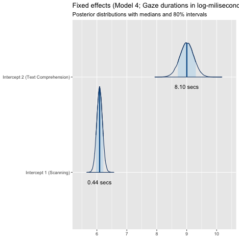
![](Earli_Sig27_2020_ninja_files/figure-html/unnamed-chunk-4-1.png)
    ]
]

---

### Posterior distribution of .pink[theta & residual variances]
.left-column[
</br>
- more visits from 'scanning' than 'text comprehension'

- residual variance larger for 'text comprehension'
]
.right-column[
  .right[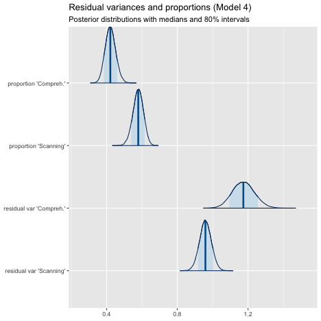
![](Earli_Sig27_2020_ninja_files/figure-html/unnamed-chunk-5-1.png)
]]
---

### Posterior distribution of .pink[random effects]
.left-column[
</br>
- judges stronger impact on both types of durations

- biggest differences for durations form 'text comprehension'
]
.right-column[
  .right[
![](Earli_Sig27_2020_ninja_files/figure-html/unnamed-chunk-6-1.png)
]]
---

### Diff. between judges in reading for text comprehension
.left-column[
</br>
_This plot shows how .pink[judges] differ in durations coming form 'text comprehension'_
]
.right-column[
  .right[
![](Earli_Sig27_2020_ninja_files/figure-html/unnamed-chunk-7-1.png)
]]
---

### Diff. between comparisons in reading for text comprehension
.left-column[
</br>
_This plot shows how .pink[comparisons] result in different durations for 'text comprehension'_

`$\rightarrow$` _clearly more alike than judges_
]
.right-column[
  .right[
![](Earli_Sig27_2020_ninja_files/figure-html/unnamed-chunk-8-1.png)
]]
---
class: inverse, center, bottom
background-image: url(felicia-buitenwerf-Qs_Zkak27Jk-unsplash.jpg)
background-size: contain
# Conclusion & Discussion

---

## Conclusion

- model that acknowledges gaze event durations come from different cognitive processes is most likely

- judges and comparisons result in different gaze event durations

- mixed effects finite mixture models are promising for this kind of data

- _no need to decide which fixation duration point to scanning and which to text comprehension_
  
  - _opens up many possibilities for follow-up research questions and analyses_

---
## Discussion

- what about more than 2 processes?

- more informed priors

- a need for .pink[triangulation] to understand the two types of processes

- what if representations are not texts; how .pink[task specific] are these models?

- other applications of .pink[(mixed effects) finite mixture models] when modelling process data?

---
class: inverse, center, bottom
background-image: url(marko-pekic-IpLa37Uj2Dw-unsplash.jpg)
background-size: contain

# Questions?

Do not hesitate to contact us!

sven.demaeyer@uantwerpen.be

The material is shared on OSF [https://osf.io/evrsf/]